
NUMERICAL SIMULATION OF HYDRODYNAMIC CHARACTERISTICS ON AN ARC CROWN WALL USING VOLUME OF FLUID METHOD BASED ON BFC*
2011-05-08 05:55LIXueyanRENBingWANGGuoYuWANGYongxue
水动力学研究与进展 B辑 2011年6期
LI Xue-yan, REN Bing, WANG Guo Yu, WANG Yong-xue
State Key Laboratory of Coastal and Offshore Engineering, Dalian University of Technology, Dalian 116023, China, E-mail: echco08@yahoo.cn
NUMERICAL SIMULATION OF HYDRODYNAMIC CHARACTERISTICS ON AN ARC CROWN WALL USING VOLUME OF FLUID METHOD BASED ON BFC*
LI Xue-yan, REN Bing, WANG Guo Yu, WANG Yong-xue
State Key Laboratory of Coastal and Offshore Engineering, Dalian University of Technology, Dalian 116023, China, E-mail: echco08@yahoo.cn
(Received May 9, 2011, Revised August 4, 2011)
In the present study, a new algorithm based on the Volume Of Fluid (VOF) method is developed to simulate the hydrodynamic characteristics on an arc crown wall. Structured grids are generated by the coordinate transform method in an arbitrary complex region. The Navier-Stokes equations for two-dimensional incompressible viscous flows are discretized in the Body Fitted Coordinate (BFC) system. The transformed SIMPLE algorithm is proposed to modify the pressure-velocity field and a transformed VOF method is used to trace the free surface. Hydrodynamic characteristics on an arc crown wall are obtained by the improved numerical model based on the BFC system (BFC model). The velocity field, the pressure field and the time profiles of the water surface near the arc crown wall obtained by using the BFC model and the Cartesian model are compared. The BFC model is verified by experimental results.
Body Fitted Coordinate (BFC), SIMPLE scheme, Volume Of Fluid (VOF) method, arc crown wall, staggered grid
Introduction
The Volume Of Fluid (VOF) method[1-4]is widely used in solving problems of viscous flows with nonlinear free surfaces or large deformations, such as the wave distortion and the wave breaking, because it is generally more efficient than the MAC method in view of computational efficiency. The classical VOF algorithm for solving the governing equations (Navier-Stokes equations)[5,6]is generally used in the Finite Volume Method (FVM), based on the Cartesian coordinate system and is useful for solving problems of simple geometries. However, some difficulties and limitations would arise in dealing with problems of complex geometries, because an orthogonal grid system might produce stepped boundaries on the solid wall boundary. With the stepped boundaries one can not accurately simulate the pressure field and the velocity field near the solid wall. Recently, a numerical approach based on the BFC system was developed to deal with this limitation[7,8].
The Body Fitted Coordinate (BFC) method was proposed by Thompson. The basic idea is that the non-uniform grid in the physical plane is transformed into a uniform, rectangular grid in the computational plane through a coordinate transform and the governing partial differential equations are solved in the uniform, rectangular computational plane. The BFC grid can accurately describe the boundaries of complex coastal structures. In the area near the solid wall, a finely spaced grid is used to deal with the large gradient of physical variables there. In the past few years, with the development of the numerical simulation methods, the VOF method, based on the BFC grid, was applied to obtain the flow field with free surfaces. Hong et al.[9]used the SIMPLE scheme, based on the non-staggered mesh, to deal with the momentum transport and the VOF method to trace the melt free surface in the mold filling processes for curved-shape or thin-walled castings. Hong[10]simulated a two-dimensional fluid flow between two plates with a semi-circular core on the bottom plate and an internal flow in a U-tube in the BFC system by the new numericalalgorithm. Huang et al.[11]developed a coupled ghost fluid/two-phase level set method by solving the twodimensional Navier-Stokes equations and the pressure Poisson equation to simulate air/water turbulent flows in complex geometries using the BFC grid. In the above non-staggered grid systems, the velocity and the pressure are calculated at the center of a control volume, which would lead to a checkerboard splitting of the pressure field known as a serious trouble in the non-staggered grid. Yuan et al.[12]proposed a numerical method to simulate the natural convection film boiling and the forced convection film boiling on a sphere under saturated conditions using the VOF method based on the BFC and adopted a double staggered grid with the SIMPLE method to solve the flow field. However, in the double staggered arrangement, the calculation of coefficients and geometrical interpolation factors is very time-consuming when different control volumes are used for different variables. The above studies were mostly for metallurgical and nuclear engineering, few for coastal engineering where such as the interactions between waves and coastal structures should be considered.
In this article, a new coupled SIMPLE algorithm with a staggered arrangement and the VOF method, based on the BFC system, is proposed to simulate fluid flows with free surfaces. The non-uniform grid in the physical plane is transformed into a uniform, rectangular grid in the computational plane through a coordinate transform and the governing partial differential equations are solved in the uniform, rectangular computational plane. Hydrodynamic characteristics[13]on the arc crown wall obtained by the BFC model are discussed. The BFC model is verified by the experimental results. The flow field, the pressure field and the time profiles of the water surface near the arc crown wall obtained by the BFC model are compared with those obtained by the Cartesian model.

Fig.1 The structure model of the arc crown wall
1. Physical model
The experiment is conducted in the oil spill tank in the State Key Laboratory of Coastal and Offshore Engineering, Dalian University of Technology. The wave channel is 23 m in length, 0.8 m in width and 0.8 m in height. The test wave is a regular wave. A wave generator driven by a servo-electro-hydraulic system is used, with a related computer control and a data acquisition system. At the far end of the tank, a wave energy dissipation device is used to attenuate the reflected waves.
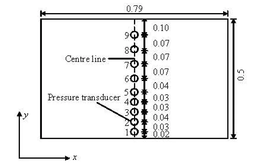
Fig.2 Pressure transducers on the surface of the arc crown wall (m)
The structure model of the arc crown wall is shown in Fig.1 and is put in the rear position of the tank. The wave pressures on the surface of the arc crown wall are measured by an SG2000 multi-point pressure measuring system, made by the Institute of Water Transportation of Tianjin. The sampling interval is 0.003 s. Nine pressure transducers are fixed on the centre line of the model surface, as shown in Fig.2. The arc crown wall is 0.5 m in height and 0.79 m in width.
2. Mathematical model
2.1 Governing equations in the BFC system
The basic governing equations for the twodimensional incompressible viscous flows are the Navier-Stokes equations and the continuity equation. The equations in the Cartesian coordinate system can be written as:
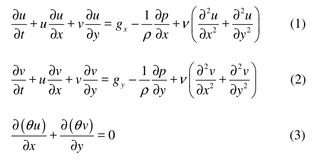
where u and v are the velocity components in the x-direction and y-direction, respectively, gxand gyare the components of the acceleration of gravity in the x-direction and y-direction, respectively, gx=− 9.8 m/s2, g=0 m/s2, p is the pressure, ρ is
y the fluid density, ρ=1000 kg/m3, ν is the coefficient of kinematic viscosity, ν =1.0× 10⁻⁶m2/s, θ is the parameter of the part cell, with a value between zero and unity.
In order to solve the governing equations in a curvilinear coordinate system, the following coordinate transformation is introduced
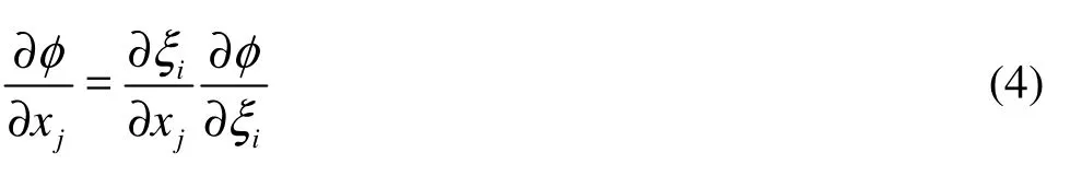
where φ is the velocity of the flow, xjis the coordinate system in the physical plane,iξ is the coordinate system in the computational plane.
With the above relations, the derivatives in the physical plane can be related to those in the computational plane as follows[14]:

Now the Navier-Stokes equations and the continuity equation in the computational plane can be rewritten as:
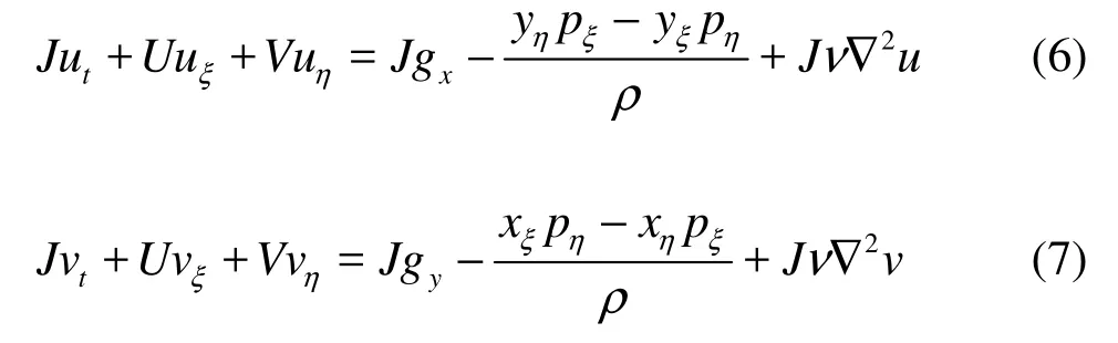

where J is the Jacobian of the transformation, uξand uηare the contravariant velocity components in the ξ-direction and η-direction, respectively.
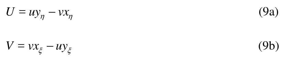
The expressions for U and V can be expressed as follows:
Equations (6)-(8) are approximated by the finite difference method, based on the staggered grid system, as shown in Fig.3. In the staggered grid system, the velocity and the pressure are calculated at the boundary and the center of a control volume, respectively, and with the interpolation method, the checkerboard splitting of the pressure field known as a serious trouble in the non-staggered grid is avoided.
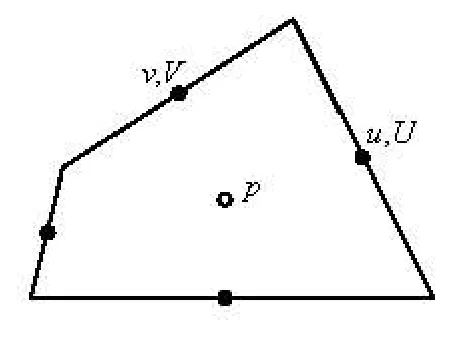
Fig.3 Configuration of a staggered grid system
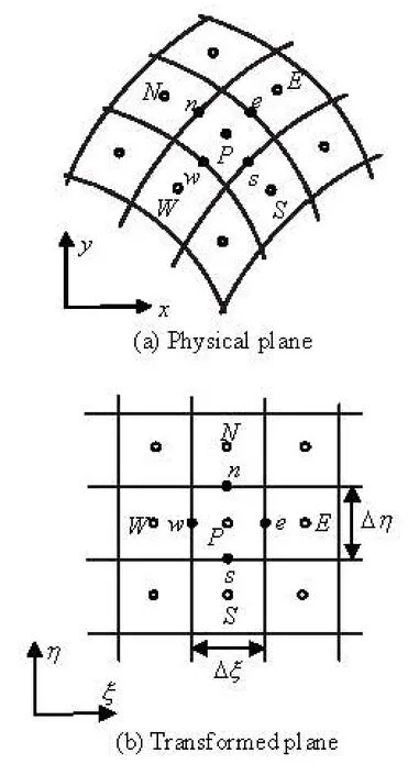
Fig.4 Finite-difference grid representation
Using the above transformation, the arbitrary geometry in the physical plane shown in Fig.4(a) is transformed into a uniform, rectangular grid in the computational plane as shown in Fig.4(b). The backward difference is used for the metric terms: xξ, xη, yξ, yη, obtained from the general transformation given by Eq.(5), the forward difference is used for the time and the central difference scheme is used for pressure and viscous terms, the nonlinear convective difference scheme is a linear combination of the oneorder upwind scheme and the second-order upwind scheme[15].
2.2 The SIMPLE algorithm in the BFC system
Ignoring the influence of the velocity corrections of the adjacent cells as are done in the Cartesian model, the velocity correction equations derived from the discrete momentum equations can be written as follows:
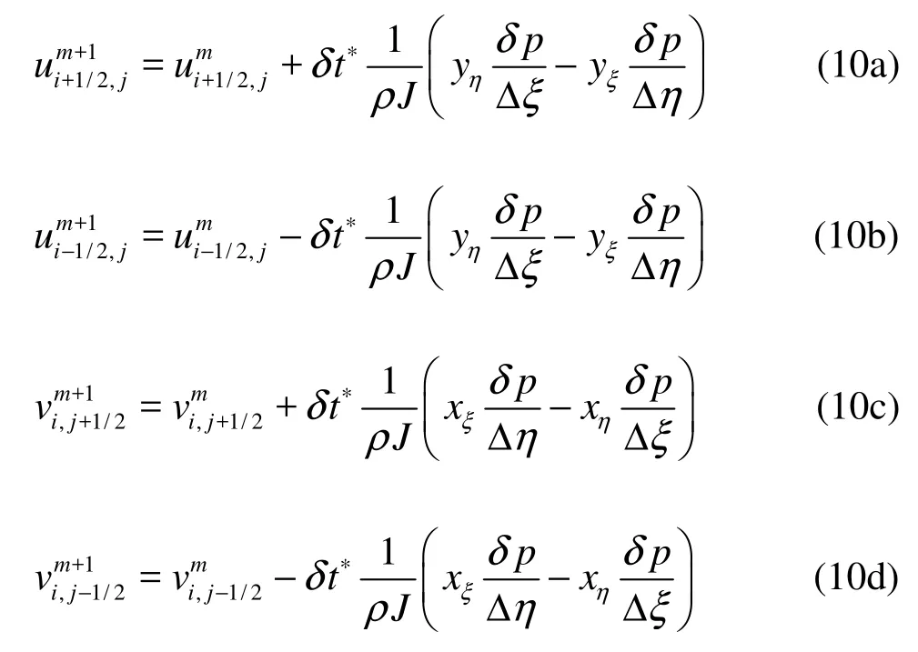
where δp is the pressure correction, xξ, xη, yξ, yηare the metric terms, respectively.
Substitution of the velocity-correction formulae into the continuity Eq.(8) yields an equation for the pressure correction as follows

where the variable s in each cell is the value of the left side of Eq.(8) in the discretized form, the residual, evaluated with the updated values of p, u and v. Pressure relaxation factor ω is adopted in Eq.(11) to improve the numerical accuracy.
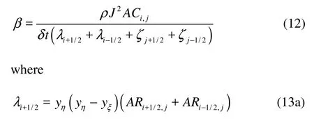
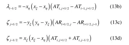
ARi+1/2,j, ARi−1/2,j, ATi,j+1/2, ATi−1,j+1/2are the fractional area coefficients open to the flow, ACi,jis the fractional volumes open to the flow. Those coefficients have an equal unit for the integral cell without any obstacle.
After solving the above pressure-correction equations, the pressure is updated by the following formula

where*
p is the pressure field before the updating.
2.3 The VOF method in the BFC system
Because the standard VOF method can not be directly applied to the BFC system, the governing equation for the fluid function F is modified for the BFC system as follows[9].
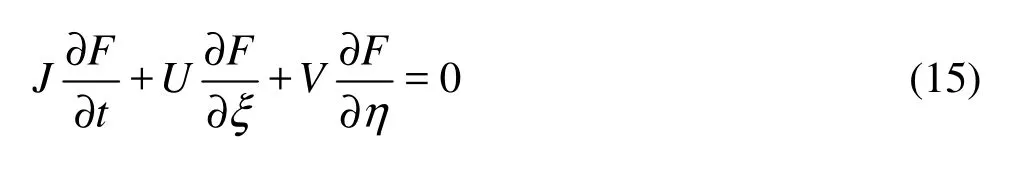
The discretized form of Eq.(15) is given by
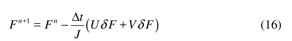
In order to preserve the smooth profile of a free surface, special care must be taken in computing the cell flux, Uδ FandVδ F. The Donor and Acceptor Flux Approximation (DAFA), usually used in the SOLA-VOF method, is adopted in the BFC model. However, the standard DAFA proposed for an orthogonal grid system cannot be used directly. The modified DAFA for a BFC grid system is given as follows[10].
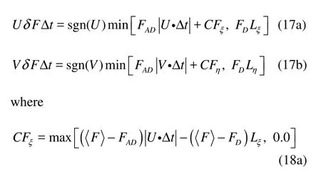
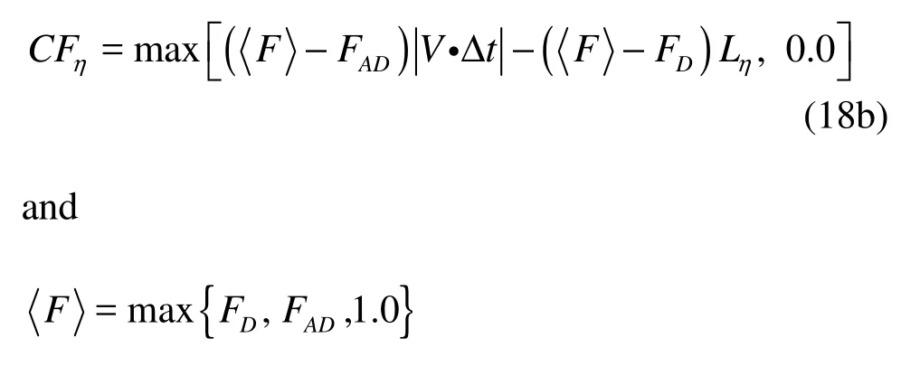
The subscript D refers to the donor cell and the subscript AD would refer to either the donor cell (D) or the acceptor cell (A), according to the directions of both the free surface and the flow. The distances Lξand Lη, and the contravariant velocity components of U and V are shown in Fig.5.
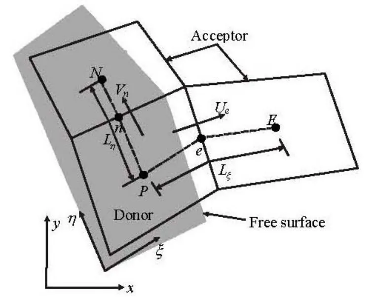
Fig.5 Notations of the donors and the acceptors in the BFC system
2.4 Pressure of a surface cell
The pressure pi,jof a surface cell in the BFC is obtained by interpolating values of its neighboring cells. The interpolation function is given by
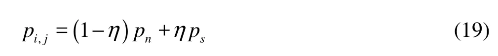
The variables in Eq.(19) are shown in Fig.6, where pnis the pressure of a neighboring cell (the interpolation cell) inside the fluid in a direction nearly perpendicular to the free surface, psis the surface pressure, computed from the surface-tension and the wall-adhesion forces, with values about zero, η= dc/d is the interpolation factor, dcis defined as a broken line distance from the center of the free surface cell to the center of the neighboring cell, as is different from the straight line distance in the Cartesian model, d is the broken line distance between the free surface cell and the center of the neighboring cell, as is also different from the straight line distance in the Cartesian model.
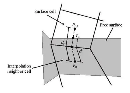
Fig.6 Evaluation of the pressure of a surface cell
3. Numerical results and discussions
The hydrodynamic characteristics on the arc crown wall are computed by the BFC model, which is verified by experimental results. The velocity field, the pressure field and the time profiles of the water surface near the arc crown wall of the BFC model obtained are compared with those of the Cartesian model.
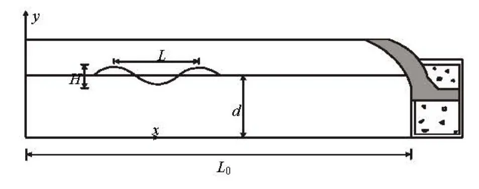
Fig.7 Sketch of the numerical wave flume with the arc crown wall
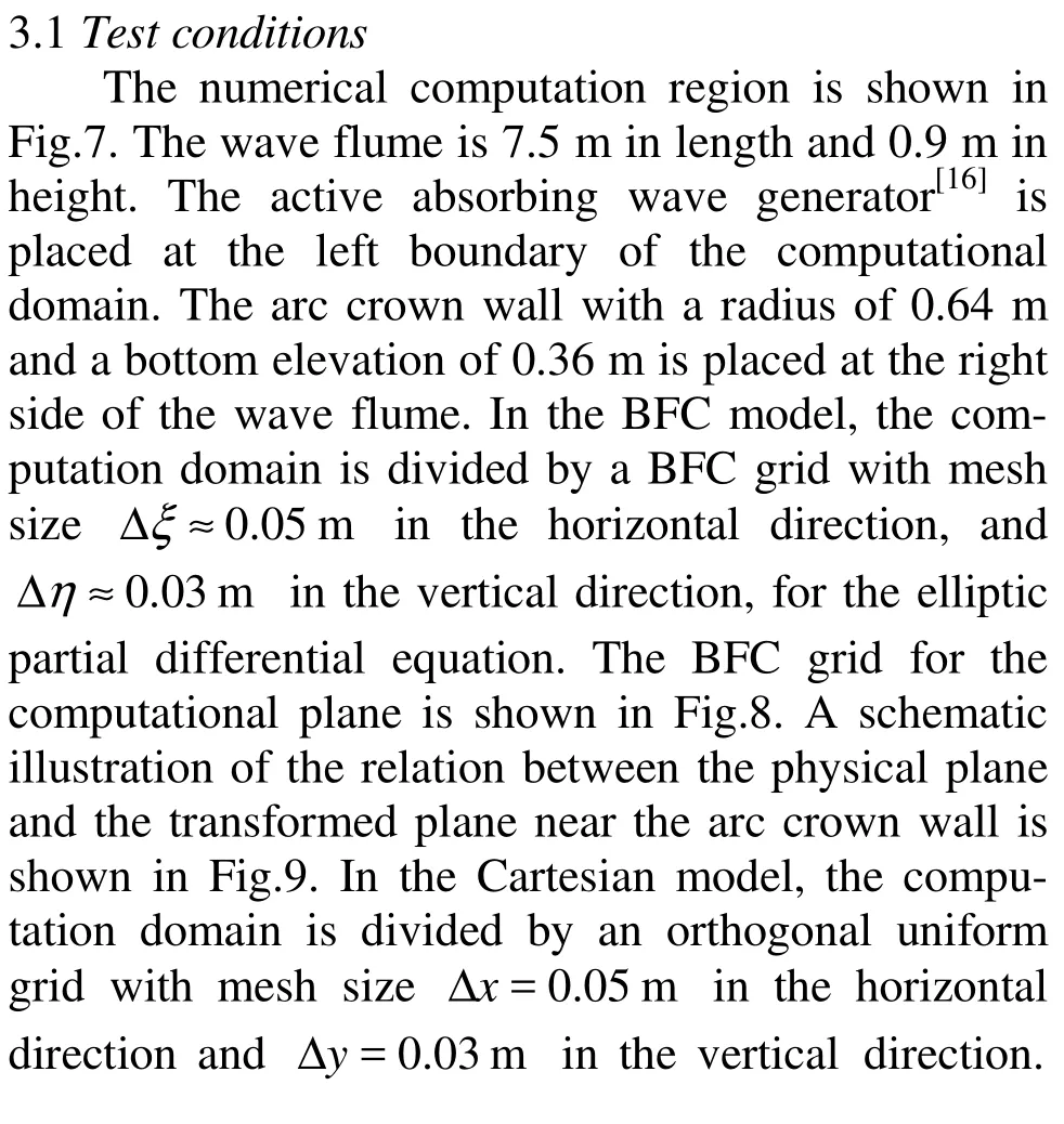
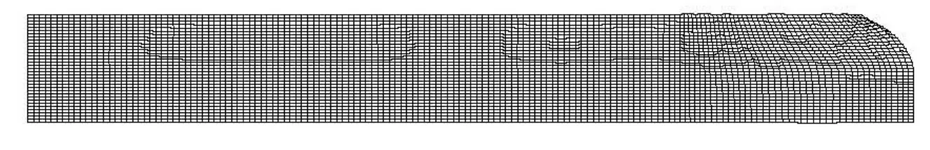
Fig.8 The grids of the numerical wave flume with the arc crown wall of the BFC model
The grid with a stepped boundary near the arc crown wall, as is treated by using the partial cell technique[17], is shown in Fig.10.

Fig.9 Coordinate transformation
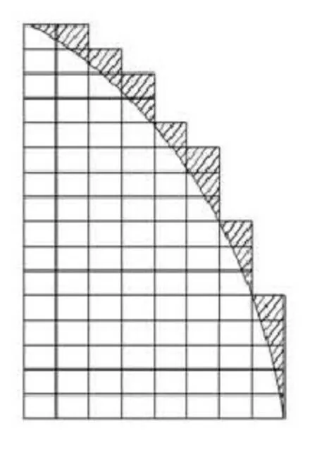
Fig.10 Grids of stepped boundaries

Fig.11 The numerical cells near the arc crown wall obtained by the BFC model
Figures 11 and 12 show the numerical cells near the arc crown wall in the BFC and the Cartesian coordinate systems, respectively. The still water level is located in the 18th cell in the vertical direction.
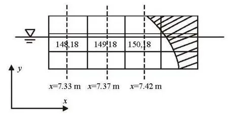
Fig.12 The numerical cells near the arc crown wall obtained by the Cartesian model
3.2 Time profiles of water surface
Figure 13 shows the comparisons between the time profiles of the water surface of the free-surface cells near the arc crown wall obtained by the BFC model and those obtained by the Cartesian model. It can be seen from Fig.13 that the wave troughs of the time profiles of the water surface obtained by the Cartesian model are rough while those obtained by the BFC model are very smooth, and the wave crests obtained by the Cartesian model are truncated at the location x =7.42 m . They might be due to the socalled stepped boundaries caused by the partial cell technique in the Cartesian model.
Figure 14 shows the comparisons of the instantaneous fluid velocities vectors at different instants near the arc crown wall for the case of T =1.5s, H= 0.11m and d =0.6 m. Figures 14(a), 14(c) and 14(e) shows the flow field obtained by the BFC model, and Figures 14 (b) 14(d) and 14(f) shows the flow field obtained by the Cartesian model. It can be seen from Fig.14, at the instant t =8.25s, a small part of water just touches the arc crown wall. At the instant t =8.75s , the water moves to the highest position of y =0.87 m on the arc crown wall. At the instant t =9.25s, most of water has dropped down. It can be also seen that the BFC results show clearly the process that the water particles climb up and drop down along the surface of the arc crown wall at various instants, while the velocity vectors of the Cartesian results nearthe arc crown wall are in a disorder, and the velocity vectors are almost in a vertical direction, not along the curving direction of the arc crown wall, which may be due to the fact that the partial cell technique is used to describe the stepped boundaries in the Cartesian model as shown in Fig.8. The velocity is defined at the boundary of the rectangular grid, not at the real boundary of the solid wall. So the Cartesian results can not truly describe the process of the water particles climbing up and dropping down along the surface of the arc crown wall.
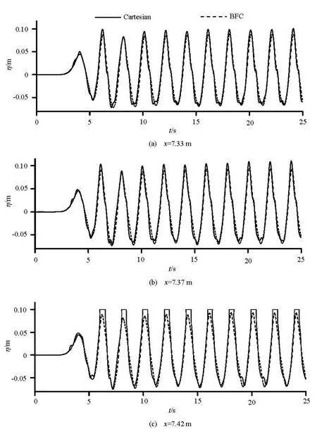
Fig.13 Time profiles of water surface near the arc crown wall (T =2.0 s , H =0.08 m , d =0.5 m )
3.4 Pressure field
Figure 15 presents the comparisons between the numerical results and the experimental data for the case of d =0.5 m , T =2.0s and H =0.08m. It is observed that the time profiles of the pressure obtained by the Cartesian model show disorders such as the collapse of gear needles and the burrs; while those obtained by the BFC model are very smooth. The numerical results are overestimated as compared with the experimental data. The disagreement might be due to the fact that the complicated turbulence dissipations in the physical test could not be fully accounted in a numerical mo de l. And it also can be seen that the wave troughsofthetimeprofilesoftheexperimentalpressure are truncated at x=0.465 m and x= 0.495 m, which is due to the fact that the underwater pressure transducers locate in positions higher than the position of the wave troughs, which will be out of water when the wave trough comes.
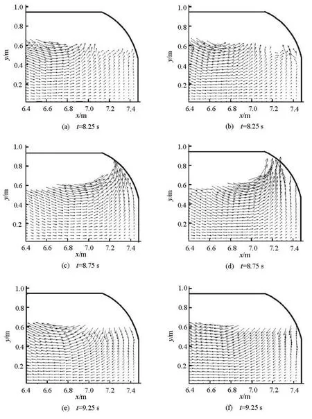
Fig.14 The comparison of local velocity fields of the arc crown wall computed by the BFC model and the Cartesian model (T=1.5s, H =0.11m , d =0.6 m )
4. Conclusions
A new coupled SIMPLE algorithm with a staggered arrangement and the VOF method based on the BFC system are proposed to deal with the interactions between the waves and the arc crown wall. The nonuniform grid in the physical plane is transformed into a uniform, rectangular grid in the computational plane by the coordinate transform method and the governing partial differential equations are solved in the uniform, rectangular computational plane. The transformed SIMPLE scheme with staggered grids and the transformed VOF method are adopted to modify the pressure-velocity field and trace the free surface, respectively. The BFC model is verified by experimental results. The flow field, the pressure field and the time profiles of the water surface near the arc crown wall obtained by the BFC model are compared with those obtained by the Cartesian model. It is concluded that with the BFC model, better results can be obtained than with the Cartesian model in simulating the interactions between the waves and the arc crown wall.
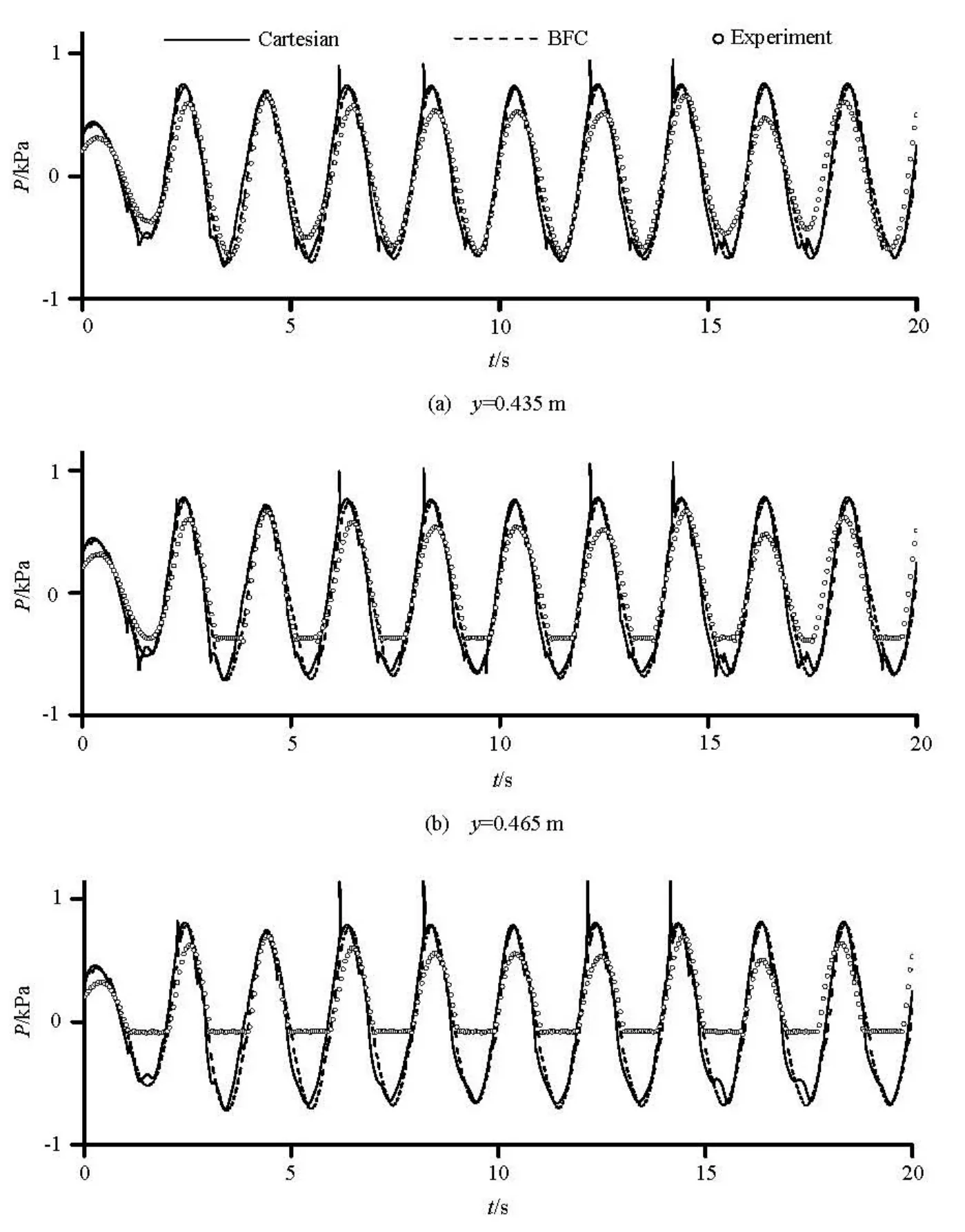
Fig.15 Time profiles of pressure near the arc crown wall ( =2.0 s T , =0.08 m H , =0.5 m d )
[1] DONG Zhi, ZHAN Jie-min. Comparison of existing methods for wave generating and absorbing in VOF-based numerical tank[J]. Journal of Hydrodynamics, Ser. A, 2009, 24(1): 15-21(in Chinese).
[2] WANG Yan-jin, FENG Qi-jing and ZHANG Shu-dao. Interface capturing method of coupled level set and VOF[J]. Chinese Journal of Hydrodynamics, 2011, 26(2): 201-208(in Chinese).
[3] DONG Zhi, ZHAN Jie-min. Numerical modeling of wave evolution and runup in shallow water[J]. Journal of Hydrodynamics, 2009, 21(6): 731-738.
[4] LI T. Q., TROCH P. and ROUCK J. D. Wave overtopping over a sea dike[J]. Journal of Computational Physics, 2004,198(2): 686-726.
移取上述适量试液(碲含量<200 μg)于25 mL比色管中,加入10 mL氢溴酸(1+1)-溴化钾(饱和),5 mL硫酸(1+1),1 mL亚铁氰化钾溶液(20 g/L),加水定容,轻摇混匀,静置30min后,用双层致密滤纸干过滤于50 mL小烧杯中,滤液用3 cm比色皿于分光光度计波长440 nm处,以试剂空白为参比,测定吸光度。随同试样做空白试验。
[5] ZHANG J. Z., REN S. and MEI G. H. Model reduction on inertial manifolds for N-S equations approached by multilevel finite element method[J]. Communications Nonlinear Science and Numerical Simulation, 2011, 16(1): 195-205.
[6] ZHOU Qin-jun, WANG Ben-long and LAN Ya-mei et al. Numerical simulation of wave overtopping over seawalls[J]. Chinese Quarterly of Mechanics, 2005, 26(4): 629-633(in Chinese).
[7] WU Shi-ping, PAN Hong and WANG Ye et al. Automatic enmeshment of 2D differential grid based on BFC (Body-fitted Coordinates)[J]. Special Casting and Nonferrous Alloys, 2011, 31(1): 25-27(in Chinese).
[8] JIANG Guang-biao, HE Yong-sen and SHU Shi. Research on generating method of the BFC grid with the adjustable boundary mesh intervals and orthodgonality[J]. Hydro-Science and Engneering, 2009, (3): 67-71(in Chinese).
[9] HONG C. P., LEE S. Y. and SONG K. Development ofa new simulation method of mold filling based on a body-fitted coordinate system[J]. ISIJ International, 2001, 41(9): 999-1005.
[10] HONG C. P. Computer modelling of heat and fluid flow in materials processing[M]. London: Taylor and Francis, 2004.
[11] HUANG J. T., CARRICA P. M. and STERN F. Coupled ghost fluid /two-phase level set method for curvilinear body-fitted grids[J]. International Journal for numerical Methods in Fluids, 2007, 55(9): 867-897.
[12] YUAN M. H., YANG Y. H. and LI T. S. et al. Numerical simulation of film boiling on a sphere with a volume of fluid interface tracking method[J]. International Journal of Heat Mass Transfer, 2008, 51(7): 1646-1657.
[13] KOUTANDOS E. V., PRINOS P. E. Hydrodynamic characteristics of semi-immersed breakwater with an attached porous plate[J]. Ocean Engineering, 2011, 38(1): 34-48.
[14] LEI C., CHENG L. and KAVANAGH K. A finite difference solution of the shear flow over a circular cylinder[J]. Ocean Engineering, 2000, 27(3): 271-290.
[15] ZHANG Cheng-xing, WANG Yong-xue and WANG Guo-yu et al. Numerical simulation study on the horizontal current generated by air bubbles curtain in still water[J]. Chinese Journal of Hydrodynamics, 2010, 25(1): 59-66(in Chinese).
[16] REN Bing, LI Xue-lin and WANG Yong-xue. Experimental investigation of instantaneous properties of wave slamming on the plate[J]. China Ocean Engineering, 2007, 21(3): 533-540.
[17] REN Xiao-zhong, WANG Yong-xue and WANG Guoyu. The irregular wave loading on the quasi-ellipse caisson[J]. Ship and Ocean Engineering, 2009, 38(1): 85-89.
10.1016/S1001-6058(10)60175-8
* Project supported by the National Natural Science Foundation of China (Grant Nos. 51179030, 50921001).
Biography: LI Xue-yan (1980-), Female, Ph. D. Candidate
REN Bing, E-mail: bren@dlut.edu.cn
猜你喜欢
小读者·阅世界(2020年6期)2020-07-29
少年文艺·开心阅读作文(2020年3期)2020-04-07
山东化工(2019年24期)2020-01-17
保健与生活(2019年6期)2019-07-31
实验技术与管理(2019年3期)2019-04-03
中国盐业(2018年17期)2018-12-23
商品与质量(2018年47期)2018-12-07
科学家(2017年8期)2017-06-22
百科知识(2016年22期)2016-12-24
中国医学装备(2015年10期)2015-12-29

- 水动力学研究与进展 B辑的其它文章
- LATTICE BOLTZMANN METHOD SIMULATIONS FOR MULTIPHASE FLUIDS WITH REDICH-KWONG EQUATION OF STATE*
- DYNAMIC ANALYSIS OF FLUID–STRUCTURE INTERACTION OF ENDOLYMPH AND CUPULA IN THE LATERAL SEMICIRCULAR CANAL OF INNER EAR*
- SIMULATIONS OF FLOW INDUCED CORROSION IN API DRILLPIPE CONNECTOR*
- NUMERICAL SIMULATION OF FLOW OVER TWO SIDE-BY-SIDE CIRCULAR CYLINDERS*
- NUMERICAL STUDY OF HYDRODYNAMICS OF MULTIPLE TANDEM JETS IN CROSS FLOW*
- EXPERIMENTAL STUDY ON SEDIMENT RESUSPENSION IN TAIHU LAKE UNDER DIFFERENT HYDRODYNAMIC DISTURBANCES*