
THERMAL IMAGING STUDY OF SCALAR TRANSPORT IN SHALLOW WAKES*
2012-05-11 06:54LIANGDongfangCHONG
水动力学研究与进展 B辑 2012年1期
LIANG Dong-fang, CHONG K. J. Y.
Department of Engineering, University of Cambridge, Cambridge, UK, E-mail: d.liang@eng.cam.ac.uk THUSYANTHAN N. I.
KW Ltd, Fetcham, Surrey, UK
TANG Hong-wu
College of Water Conservancy and Hydropower Engineering,, Hohai University, Nanjing 210098, China
THERMAL IMAGING STUDY OF SCALAR TRANSPORT IN SHALLOW WAKES*
LIANG Dong-fang, CHONG K. J. Y.
Department of Engineering, University of Cambridge, Cambridge, UK, E-mail: d.liang@eng.cam.ac.uk THUSYANTHAN N. I.
KW Ltd, Fetcham, Surrey, UK
TANG Hong-wu
College of Water Conservancy and Hydropower Engineering,, Hohai University, Nanjing 210098, China
(Received April 19, 2011, Revised July 15, 2011)
The thermal imaging technique relies on the usage of infrared signal to detect the temperature field. Using temperature as a flow tracer, thermography is used to investigate the scalar transport in the shallow-water wake generated by an emergent circular cylinder. Thermal imaging is demonstrated to be a good quantitative flow visualization technique for studying turbulent mixing phenomena in shallow waters. A key advantage of the thermal imaging method over other scalar measurement techniques, such as the Laser Induced Fluorescence (LIF) and Planar Concentration Analysis (PCA) methods, is that it involves a very simple experimental setup. The dispersion characteristics captured with this technique are found to be similar to past studies with traditional measurement techniques.
environmental hydraulics, shallow wake, turbulent mixing, thermal imaging, vortex street
Introduction
Shallow flows, i.e., flows with horizontal dimensions much larger than their vertical dimensions, are ubiquitous in the environment. The flow in wide river channels, lakes, estuaries, coastal zones, surface-water runoff or stratified atmosphere can all be classified as shallow one[1]. Topographical forcing in the form of islands, vegetations, bridge piers or wide working platforms can lead to the formation of a wake envelope of von Kármán vortices. While the limited flow depth restricts the development and movement of these vortices in the vertical direction, lateral instabilities are free to propagate in the horizontal plane and acquire quasi two-dimensional (2-D) features. These large flow structures play an important role in the exchange of momentum, mass and heat in the flow.
The study of turbulent mixing phenomena in shallow waters is relevant to many environmental engineering applications. When chemicals are introduced into water, depending on the situations, there exists a need to either enhance or suppress the mixing. A better understanding of the scalar transport process in shallow waters is needed to minimize the detrimental effects of an oil or chemical effluent spill on the aquatic ecosystem. There have been many studies dedicated to investigating the turbulent mixing processes in the shallow wakes of bluff bodies[1-6]. These studies all used certain tracer materials to mark the scalar quantity. Since temperature is a scalar quantity subject to ambient fluid convection, the development of the temperature field should also exhibit characteristics similar to those of the development of the material concentration field.
Significant strides made in video imaging technology have witnessed the development of various non-intrusive quantitative flow visualization techniques such as the Particle Image Velocimetry (PIV), Planar Concentration Analysis (PCA) and Laser Induced Fluorescence (LIF) methods. Of these, LIF andPCA have been used to obtain the scalar field by measuring the concentration of a tracer substance. For the LIF technique, laser is used to excite dissolved dye tracer, which emits fluorescent light at a different frequency and wavelength to the source laser beam with the intensity related to the concentration of the tracer[7]. The PCA technique relies on the variation of the solute color with the dye concentration to quantify the scalar transport process[2,3]. In studies of shallow flows, the PCA technique is often used to measure the concentration field from above the free surface, yielding effectively depth-integrated values. The variation of concentrations over the depth is assumed to be negligible relative to the changes along the horizontal directions.
In this study, the feasibility of using thermal imaging to investigate the scalar transport process in shallow wakes is explored. Although thermal imaging in itself is not a novel technology, its usage in quantitative measurement in fluid mechanics has been rare. Past studies on heat transfer in the wake of a bluff body have utilized hot-wire anemometry[8]and platinum wire resistance thermometers[9], where temperature fluctuations at discrete points were measured in air flows. The fragility of the thin probes renders them unsuitable for use in a much denser medium such as water. In water flows, the extent of flow intrusion increases with the utilization of thicker hot-film probes instead[10]. By contrast, thermal imaging captures the instantaneous two-dimensional temperature field without any intrusion.
In this experiment, the temperature difference is created by injecting warm water into the ambient fluid at room temperature directly behind a cylinder. The entrainment of warm water in the von Kármán vortex street is then be distinguished by deploying an infrared camera. A key attraction of the thermal imaging method over other scalar measurement techniques, such as the LIF and PCA methods, is that it involves a much simpler setup. Moreover, since the tracer for the thermal imaging technique is fluid-based, the issue of particle agglomeration, often associated with some of the other quantitative flow visualization techniques, is avoided.
1. Thermal imaging technique
A Mobir M4 infrared camera, which has a video capture rate of 25 Hz and a resolution of 19 200 pixels (160×120 pixels), is used for quantitative flow visualization in the present study. The temperature of an object, T, is calculated using the Stefan-Boltzmann law for blackbody radiation

whereobjI is the power radiated by an object of area A, ε is the emissivity of the object and σ is the Stefan-Boltzmann constant.
From a practical grey body, the signal detected by the camera is a combination of the energy emitted by the object itself, energy reflected from surrounding bodies, the buffer of the intermediate air separating the camera and the objects, and the contribution from the camera’s inner optics[11]. However, the camera is designed to automatically compensate for the effects attributed to optical transmission, and the equation for the measured radiation intensity,measI can be expressed as follows

where surr I , atm I and τ are power reflected from surrounding objects, atmospheric radiation and the atmospheric transmission coefficient respectively, surr I and atm I are estimated by the camera. Then, the input of values for τ and ε enables the camera to correct for radiation not attributed solely to the target object, and thus a value for T can be decided using Eqs.(1) and (2).
According to Rainieri and Pagliarini[11], the quality of thermal images has been substantially improved with the introduction of focal plane array sensors in replacement of the conventional single sensor thermal imaging technology. Even with this innovation, nonuniformity of the photo sensor array still poses an impediment to the performance of modern infrared cameras. Non-uniformity errors are introduced when a highly diffused image is measured by a linear array photo sensor that has been calibrated in a specular mode, manifesting themselves as unexpected streaklines in the captured image. Non-uniformity errors are not an issue when the camera is used to capture still images, as a pixel-by-pixel calibration can be performed just before a picture is taken. When the camera is operating in the video mode though, the camera automatically calibrates itself until a prescribed tolerance for non-uniformity errors of ±2% has been reached. An infrared camera with a smaller error tolerance will have to perform self-calibrations more frequently during the video recording, through which high accuracy is achieved.
Image snapshots can be extracted from a video footage recorded by the camera at specified time intervals using video processing software. The captured flow images are composed of color pixels, which can be converted into greyscale images. A calibration curve in the present study relates the greyscale level to the corresponding temperature over a particular temperature range. The temperature range in this study isfixed at 18°C to 27°C, giving a measured resolution of 0.035°C. A smaller temperature range would give a higher temperature resolution. However, this range has been carefully chosen so that the maximum and minimum temperature values measured for all experiments in this study falls within the prescribed range, and no saturation occurs. Figure 1 demonstrates the approximately linear relationship between greyscale level and temperature.

Fig.1 Relationship between greyscale levels and temperatures

Fig.2 Sketch of the top and side views of the water channel
2. Experimental setup and procedure
Experiments in the present study are conducted in a hydraulic flume, which is 2.1 m long and 0.6 m wide, filled with water to a depth of 0.045 m to represent shallow flow conditions. The free-stream velocity U is set to 0.035 m/s in this study. Figure 2 provides the top view and side view of the water channel and the definition of coordinates, with d and h being the cylindrical diameter and flow depth respectively. The honeycomb flow straighteners at the entrance of the water channel help to remove inflow non-uniformities. d should not be a significant proportion of the channel width, or the resulting wake may interact with the channel walls, generating undesirable complications. Using d=0.002 m yields a blockage factor of 3.3%, which is less than half the blockage in the experiments by Balachandar et al.[2]
By taking the kinematic viscosity coefficient of water to be 1.004×10⁻⁶m2/s, the Reynolds number based on the bluff body diameter697. For shallow wakes, Jirka[1]introduced a nondimensional wake stability number, S given in Eq.(3), which is effectively a measure of the relative significance between bed friction and lateral shear.

where the skin friction coefficientfC can be estimated using the following formula recommended by Carter et al.[12]for a smoothed turbulent boundary flow

In past studies of temperature fields behind bluff bodies[8,9], where air was taken as the working fluid, the bluff body was heated up and the heat influx was convected downstream by the moving air. However, when water, which has a heat capacity approximately four times of that for air, is used, a more concentrated heat input method is required to achieve an ideal temperature range for the measurement. In this study, hot water housed inside a container elevated at a height of 0.3 m above the channel water surface is siphoned out through a plastic tube with an inner diameter of 0.005 m and discharges into the ambient flow immediately downstream of the bluff body. The hot water tube is vertically embedded into a small slot on the rear surface of the bluff body to limit the disturbance to the flow. Small holes are drilled uniformly along the submerged part of the tube, which acts as a line source to release warm water uniformly over the depth. The volumetric flow rate of hot water, which is greatly influenced by the container height and tube diameter, should not be too high to severely interferewith the ambient flow, and neither should it be too low such that the camera can hardly distinguish the temperature difference during mixing. A trade-off has been made, and it is found that a volumetric flow rate at the tube outlet of 5.56×10⁻⁶m3/s gives a good experimental outcome in this study. Similar experimental configuration has also been adopted by Balachandar et al.[2]
A hot water temperature of 85°C is used to achieve the best effect in measurements. There is only roughly a 2.8% difference in density between the ambient water at 19°C and the hot water tracer at 85°C, so the thermal buoyancy influence is not significant for short-distance measurements. Moreover, the hot water cools down immediately after being released into cold water due to the rapid mixing. The greaterthan-unity Prandtl number for liquid water indicates that the thermal diffusivity of liquid water is smaller than its molecular viscosity. This factor, coupled with the fact that turbulent diffusion and dispersion dominate over molecular diffusion in turbulent flows, makes temperature a good indictor for studying turbulent mixing characteristics.
The infrared camera is mounted at a height of 2 m above the water surface, yielding a projected measurement area of 0.8 m×0.6 m, and a spatial resolution of 0.004 m per pixel. This is a compromise between achieving a high spatial resolution and covering a large measurement area. The rate at which flow images are extracted from the video footage is set at 6.25 Hz, giving a temporal resolution more than two times higher than that used by Balachandar et al.[3]in their study of dye concentration fields. When a sequence of instantaneous temperature distributions has been extracted, mean values and other statistical parameters can be calculated. It has been found that 200 flow images are generally needed for the mean temperature calculations to converge, giving a total sampling time of 32 s and corresponding to at least three vortex shedding cycles in this study.

Fig.3 Snapshot image obtained by thermal camera
Figure 3 shows a typical snapshot from the camera, which clearly illustrates vortex shedding immediately downstream of the cylinder, with the flow moving from top to bottom in the picture. The entrainment of hot and cold water by vortices results in regions of different temperatures, with whitish hues representing warm regions and blackish hues representing cold regions. It is also apparent that largescale vortices are aligned on both sides of the wake centreline in an alternating fashion.
3. Results and discussion
3.1 Average temperature distribution
The mean temperature,meanT, is obtained by

where N represents the length of time series.

Fig.4 Mean temperature
Figure 4(a) is the mean temperaturemeanT contour over the measurement area, whereambT represents the ambient temperature. Figure 4(b) displays the mean lateral temperature profiles taken at five different downstream sections of the cylinder. Despite having only one peak, the steep variations disallow a Gaussian fit. Instead, the composite exponential function of Eq.(6), similar to the form used by Balachandar et al.[2], has been plotted to demonstratethe trend of variation, where parameters1P to5P are decided according to the least-squares criterion and their values vary from curve to curve. It is clear from Fig.4 that the mean temperature at wake centreline (/=0yd) decreases continuously in the downstream direction. However, the mean temperature some distance away from the centerline appears to increase with downstream distance, as the lateral temperature profile flattens.

Figure 4(a) also exhibits that even when a hot water temperature of 85°C is injected, the mean temperature difference at regions near x/d=30 is only a mere 2°C. This highlights a challenge of using temperature as a flow marker for fluids with a high heat capacity. The rapid transfer of heat renders the reduction of flow structures at far wakes extremely difficult, as temperature difference diminishes quickly with the increasing downstream distance.

Fig.5 Streamwise variation of the wake half-width
The half-width T δ of temperature wake is defined as the lateral offset from the wake centreline, for which temperature is half of the maximum value at a given downstream section. Figure 5 shows that T δ increases monotonically following the 1/2 T δ ∝ x relationship as proposed by Taylor[13], and is able to reach a size of up to eight times the cylindrical diameter within the measurement domain. The effect of bed friction grows downstream relative to shear instability. The growth and motion of the large horizontal vortices are increasingly retarded with the downstream distance, and the turbulent kinetic energy produced by transversal shearing of the mean flow is converted into small three-dimensional eddies by bed friction. As is evidenced in Fig.5, the 1/2 T δ ∝ x law is on the verge of breakdown at very large values of x / d . These results have been corroborated by the decreased expansion rate of the concentration wake half-width in previous researches[2,3].

Fig.6 Maximum, mean and minimum temperatures at /=x d 4

Fig.7 A typical sequence of thermal images
3.2 Instantaneous temperature distribution
Whilst mean temperature can be used to gauge the average mixing characteristics, information on the maximum temperature may be useful particularly in real-life environmental problems, where it has to ensure that the maximum concentration of a chemical is kept at a level small enough to pose no serious harm to organisms. Figure 6 shows that the maximum temperature at certain lateral positions in the cross-section x / d = 4 can be larger than twofold of the corresponding average value. A large disparity between the mean and instantaneous scalar quantities has also been mentioned by Jiang et al.[7] in their study of lateral concentration profiles. Figure 7 further elucidates this point, where well-organized vortex street is seen and the instantaneous temperature at a position marked with “ + ” varies significantly with time. In addition,Fig.6 shows that the absolute difference between the maximum and mean temperatures is particularly large close to the wake centerline, where turbulent intensity is high.

Fig.8 Root-mean-square temperature distribution
3.3 Root-mean-square temperature distribution
The root-mean-square (rms) temperature,rmsT is given by

It is evident from Fig.8(a) that the rms temperature appears to be generally symmetrically distributed about the wake centerline. Double peaks can be observed in the lateral rms temperature profiles of Fig.8(b), which, alongside with Fig.7, signifies the presence of strong unsteady flows. The instantaneous temperature reaches a local maximum at the vortex centre, because the released hot water is wrapped inside as the incoming cold water passes the cylinder. As the Kármán vortices travel downstream, the vortices continue to entrain the surrounding fluid and grow in size, leading to a drop in the temperature difference between the vortex center and the surroundings. It is evident that the separation of the double peaks enlarges and the fluctuation of the temperature weakens with downstream distance. Equation (6) also provides a fairly good fit to the lateralrmsT profiles, especially over the range 0/8xd≤≤.
3.4 Periodicity studies
The flow integral length scale based on temperature,TL, which is essentially a measure of the size of the largest eddies, is given by

where the autocorrelation function of temperature at a spatial offset of xΔ is defined as


Fig.9 Spatial variations of temperature along /=4y d
Figure 9 displays two examples of the temperature fluctuation profile at two instants, 1 t (1.76 s) and 2 t (17.76 s), from which the spatial autocorrelation are conducted and plotted in Fig.10. The spatial autocorrelation coefficient ( ) T R Δx is computed up to only Δx / d = 22 , which corresponds to roughly three quarters of total available data length, as practiced by Mansy et al.[14] Further increasing Δx means that the data points used in calculating the two-pointcorrelation are too few to get a reliable RT(Δx).

Fig.10 Spatial autocorrelation of temperature fluctuations along y/ d=4
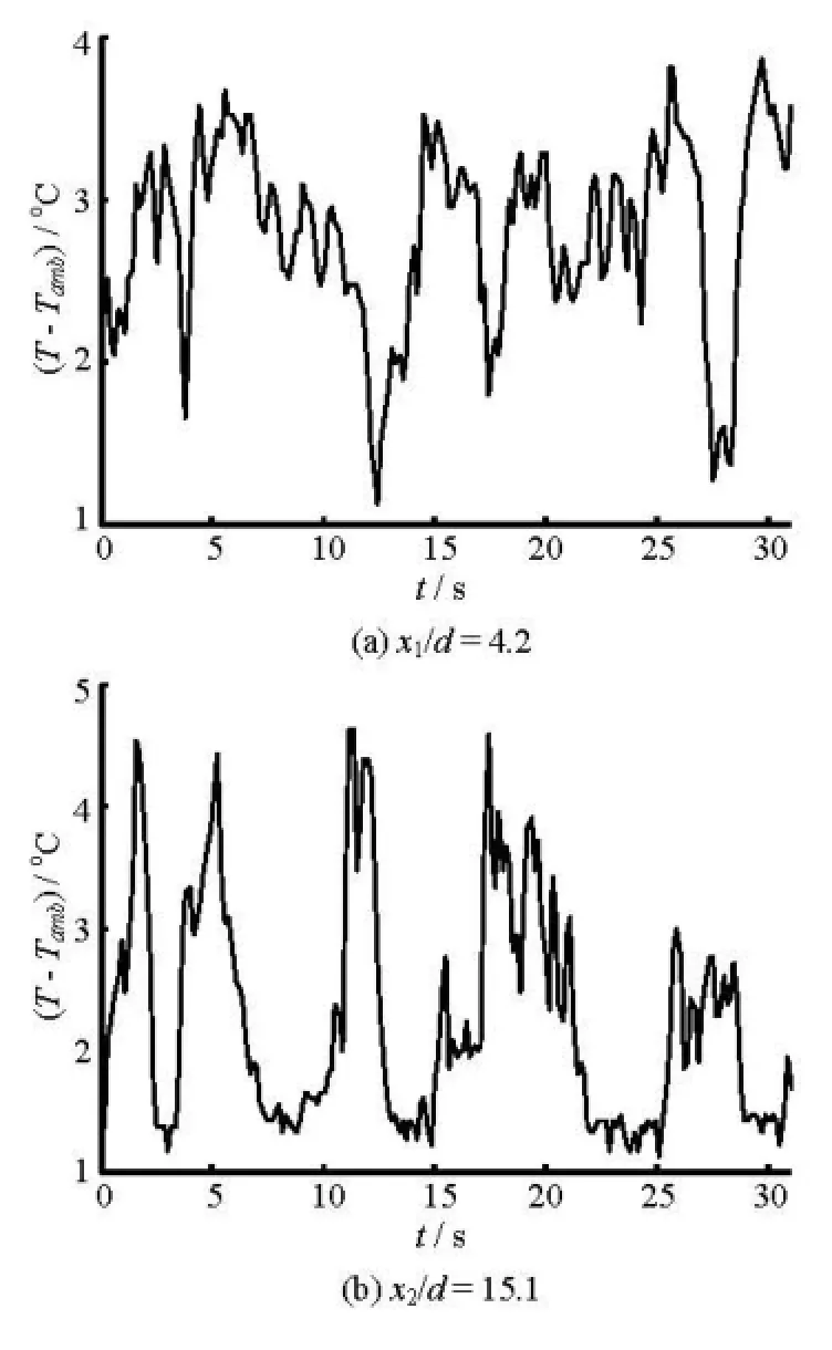
Fig.11 Time series of temperature at /=4y d
In wake flows, strong periodicity can be observed in ( ) T R x Δ , as Fig.10 shows. By comparing the regular oscillatory behaviour of Figs.10(a) and 10(b), there exist two different characteristic streamwise wavelengths χ λ : 6.0d at 1 t and 8.4d at 2 t . Since wavelength is inversely proportional to frequency by assuming that the flow structures travels downstream at a constant speed, this implies that the vortex shedding frequency at 2 t is 5/7 of that at 1 t (i.e., 2 1 f = 5 f / 7 ). The presence of a subharmonic frequency suggests the possible occurrence of vortex pairing in the shear layer, by which larger vortices with slower travelling speed are created[15]. Applying Eq.(8) to the flow at 1 t yields a flow integral length scale of around = 0.02m T L , which is equal to the cylindrical diameter.

Fig.12 Temporal autocorrelation of temperature fluctuations at y/ d=4
Analogous to the definition of Eq.(8), the flow integral time scale based on the temperature measurement,TT, is given by

where the autocorrelation function of temperature at a temporal delay of tΔ is defined as

The time series data of Fig.11 is used to generate the temporal autocorrelation of temperature fluctuations at two different downstream sections, x1/d= 4.2 and x2/d=15.1 inside the measurement area. Similar to the case of the spatial autocorrelation coefficient RT(Δx), the temporal autocorrelation coefficient RT(Δt) varies regularly as shown in Fig.12. Comparing the number of full oscillation over a fixed time offset Δt confirms the previous observations that there exists two frequencies in the flow, which differ from each other by a factor of 5/7. Using Eq.(10), the integral time scale is found to be TT= 0.6s. The ratio of LTto TTgives 0.0333 m/s, which is fairly close to the freestream velocity of 0.035 m/s used in this experiment.
4. Conclusion
The main purpose of this article is to demonstrate that the thermal imaging technique is a viable quantitative flow visualization technique for studying shallow turbulent mixing properties. Mean temperature, rms temperature and autocorrelation studies have been conducted concerning the shallow-water wake of a circular cylinder. The current experimental results basically agree with the past studies using traditional measurement techniques. The lack of complicated experimental setup and calibration procedures and the absence of tracer particle agglomeration problems, often encountered by many widely-used dye-concentration measurement methods, are the key attractions of this technique. However, non-uniform plane array issues and rapid diminishment of temperature difference in fluids with high heat capacity leaves room for future improvement in applying the thermal imaging technology.
[1] JIRKA G. H. Large scale flow structures and mixing processes in shallow flows[J]. Journal of Hydraulic Research, 2001, 39(6): 567-573.
[2] BALACHANDAR R., CHU V. H. and ZHANG J. Experimental study of turbulent concentration flow field in the wake of a bluff body[J]. Journal of Fluids Engineering, 1997, 119(2): 263-270.
[3] BALACHANDAR R., TACHIE M. F. and CHU V. H. Concentration profiles in shallow turbulent wakes[J]. Journal of Fluids Engineering, 1999, 121(1): 34-43.
[4] LIANG Dong-fang, LI Yu-liang and CHEN Jia-fan. Experimental study of shallow wake flow of plate peninsula[J]. Experiments and Measurements in Fluid Mechanics, 2004, 18(1): 15-19(in Chinese).
[5] LIANG Dongfang, LI Yu-liang and CHEN Jia-fan. Experimental study on near field shallow wake flow of peninsula[J]. Progress in Natural Science, 2004, 14(4): 431-435(in Chinese).
[6] Von CARMER C. F. Shallow turbulent wake flows: Momentum and mass transfer due to large-scale coherent vortical structures[D]. Ph. D. Thesis, Karlsruhe, Germany: University of Karlsruhe, 2005.
[7] JIANG Chun-bo, LI Yu-liang and Liang Dong-fang et al. Experimental study of steady concentration fields in turbulent wakes[J]. Experiments in Fluids, 2001, 31(3): 269-276.
[8] MATSUMURA M., ANTONIA R. A. Momentum and heat transport in the turbulent intermediate wake of a circular cylinder[J]. Journal of Fluid Mechanics, 2006, 250: 651-668.
[9] LARUE J. C., LIBBY P. A. Temperature fluctuations in the plane turbulent wake[J]. Physics of Fluids, 1974, 17(11): 1956-1967.
[10] BRUUN H. H. Hot-film anemometry in liquid flows[J]. Measurement Science and Technology, 1996, 7(10): 1301-1312.
[11] RAINIERI S., PAGLIARINI G. Data processing technique applied to the calibration of a high performance FPA infrared camera[J]. Infrared Physics and Technology, 2002, 43(6): 345-351.
[12] CARTER R. W., EINSTEIN H. A. and HINDS J. et al. Friction factors in open channels: Progress report of the task force on friction factors in open channels of the committee on hydro-mechanics of the hydraulics division[J]. Journal of the Hydraulics Division, 1963, 89(2): 97-143.
[13] TAYLOR G. I. The transport of vorticity and heat through fluids in turbulent motion[J]. Proceedings of the Royal Society of London Series A, 1932, 135(828): 685-702.
[14] MANSY H., YANG P. and WILLIAMS D. R. Quantitative measurements of three-dimensional structures in the wake of a circular cylinder[J]. Journal of Fluid Mechanics, 2006, 270: 277-296.
[15] RAJAGOPALAN S., ANTONIA R. A. Flow around a circular cylinder—structure of the near wake shear layer[J]. Experiments in Fluids, 2005, 38(4): 393-402.
10.1016/S1001-6058(11)60214-X
* Project supported by the Non-profit Public Research Project of Ministry of Water Resources (Grant No. 200901005), the National Natural Science Foundation of China (Grant No. 50879019), and the Research Fund for Doctoral Program of Higher Education (Grant No. 200802940001).
Biobraphy: LIANG Dong-fang (1975-), Male, Ph. D., Lecturer
2012,24(1):17-24

- 水动力学研究与进展 B辑的其它文章
- WALL EFFECTS ON FLOWS PAST TWO TANDEM CYLINDERS OF DIFFERENT DIAMETERS*
- A NOVEL DESIGN OF COMPOSITE WATER TURBINE USING CFD*
- ANISOTROPIC PERMEABILITY EVOLUTION MODEL OF ROCK IN THE PROCESS OF DEFORMATION AND FAILURE*
- HIGH-SPEED FLOW EROSION ON A NEW ROLLER COMPACTED CONCRETE DAM DURING CONSTRUCTION*
- THE SLOP FLUX METHOD FOR NUMERICAL BALANCE IN USING ROE’S APPROXIMATE RIEMANN SOLVER*
- BLADE SECTION DESIGN OF MARINE PROPELLERS WITH MAXIMUM CAVITATION INCEPTION SPEED*