Snow water equivalent over Eurasia in the next 50 years projected by aggregated CMIP3 models

LiJuan Ma , Yong Luo , DaHe Qin

1. National Climate Center, Beijing 100081, China 2. Center for Earth System Science, Tsinghua University, Beijing 100084, China 3. China Meteorological Administration, Beijing 100081, China 4. State Key Laboratory of Cryospheric Sciences, Cold and Arid Regions Environmental and Engineering Research Institute,Chinese Academy of Sciences, Lanzhou, Gansu 730000, China

Snow water equivalent over Eurasia in the next 50 years projected by aggregated CMIP3 models

LiJuan Ma1*, Yong Luo2, DaHe Qin3,4

1. National Climate Center, Beijing 100081, China 2. Center for Earth System Science, Tsinghua University, Beijing 100084, China 3. China Meteorological Administration, Beijing 100081, China 4. State Key Laboratory of Cryospheric Sciences, Cold and Arid Regions Environmental and Engineering Research Institute,Chinese Academy of Sciences, Lanzhou, Gansu 730000, China

Based on remote sensing snow water equivalent (SWE) data, the simulated SWE in 20C3M experiments from 14 models attending the third phase of the Coupled Models for Inter-comparison Project (CMIP3) was first evaluated by computing the different percentage, spatial correlation coefficient, and standard deviation of biases during 1979-2000. Then, the diagnosed ten models that performed better simulation in Eurasian SWE were aggregated by arithmetic mean to project the changes of Eurasian SWE in 2002-2060. Results show that SWE will decrease significantly for Eurasia as a whole in the next 50 years. Spatially, significant decreasing trends dominate Eurasia except for significant increase in the northeastern part. Seasonally, decreasing proportion will be greatest in summer indicating that snow cover in warmer seasons is more sensitive to climate warming. However, absolute decreasing trends are not the greatest in winter, but in spring. This is caused by the greater magnitude of negative trends, but smaller positive trends in spring than in winter. The changing characteristics of increasing in eastern Eurasia and decreasing in western Eurasia and over the Qinghai-Tibetan Plateau favor the viewpoint that there will be more rainfall in North China and less in the middle and lower reaches of the Yangtze River in summer. Additionally, the decreasing rate and extent with significant decreasing trends under SRES A2 are greater than those under SRES B1, indicating that the emission of greenhouse gases (GHG) will speed up the decreasing rate of snow cover both temporally and spatially. It is crucial to control the discharge of GHG emissions for mitigating the disappearance of snow cover over Eurasia.

snow water equivalent; projection; CMIP3; Eurasia; climate change; simulation

1. Introduction

Projection of global climate is currently one of the key issues of studies on climate change. In terms of ice mass and its heat capacity, the cryosphere is the second largest component of the climate system (Lemkeet al., 2007). It is garnering unprecedented attention due to its rapid and noteworthy response to and impacts on climate change. Snow cover is one of the main components of the cryosphere, and is one of the most rapidly changing types on land. With features of high albedo, high latent heat in phase transition, and low heat conduction, snow cover plays an important role in exchange of energy, mass, and water between the land surface and the atmosphere. Also, it is a non-ignorable indicator for climate prediction.

Eurasia is an important continental-scale region in the Northern Hemisphere. Snow cover over Eurasia not only has important impacts on climate in China (Wuet al., 2009),but also is an important solid water resource that residents in Asian arid and semi-arid areas live by. Changes of snow cover are the embodiment of climate change. Under the circumstance of exacerbating future climate warming,changes of Eurasian snow cover deserve special attention.Over the years, numerous researchers performed studies on projecting climate change on a global and regional scale during the next 50-100 years, which includes the projection of typhoons (Zhaoet al., 2007a; Murakami and Wang,2010), glaciers (Shi and Liu, 2000) and water resources(Shi, 2001) in western China, global and Chinese precipitation (Dinget al., 2007; Zhaoet al., 2008), and air temperature and precipitation in the middle and lower reaches of the Yangtze River (Xuet al., 2004), the Qinghai-Tibetan Plateau (Xuet al., 2003a), and northwestern China (Xuet al., 2003b, c; Zhaoet al., 2003). Zhaoet al.(2007b)summed up the projection results of air temperature reported by the Intergovernmental Panel on Climate Change(IPCC) since 1990, including the Fourth Assessment Report (AR4) and the supplementary report of the First Assessment Report (FAR). Thus, most studies focused on the projection of main parameters in the atmosphere,i.e., air temperature and precipitation, but less on cryospheric parameters. Considering the important role of the cryosphere in the climate system and the significant impacts of Eurasian snow cover on precipitation during flood seasons in China, it is crucial to project future changing characteristics of Eurasian snow cover under higher and lower emission scenarios of greenhouse gases (GHG). This will not only help project changes of water resources and ecology on both continental and regional scales, but also further provide physical scientific basis for policy decisions to adapt to and mitigate climate change.

IPCC AR4 summed up studies on snow cover and global change, and pointed out that snow cover reflected both changes of air temperature and precipitation and there was significant negative correlation between snow cover and air temperature. Results from models attending IPCC AR4 projected that snow cover in the Northern Hemisphere will decrease on a large scale in the 21st century (Meehlet al., 2007)except for some regions,e.g., Siberia, where snow cover will increase due to possible increase in autumn and winter precipitation (Meleshkoet al., 2004; Hosakaet al., 2005).Additionally, multi-model ensemble results from the Arctic Climate Impact Assessment (ACIA) indicate that annual mean snow cover in the Northern Hemisphere will decrease by 13% under higher GHG emission scenario (SRES A2) at the end of the 21st century (ACIA, 2004), and the decreasing rates range from 9% to 17% projected by any single model among them. It has been disclosed that snow cover decreases most in spring, late autumn and early winter,which means a shorter snow cover duration (ACIA, 2004).Projection results also disclosed a decrease of snow cover fraction besides the future shortening of snow cover duration(Hosakaet al., 2005). Therefore, this study initially validated the ability of IPCC AR4 models on simulating snow water equivalent (SWE) over Eurasia in the 20th Century Climate in Coupled Climate Models (20C3M) experiment by using remote sensing (RS) data during 1979-2000. Subsequently,results from models with better performance under SRES A2 and B1 (lower GHG emission scenario) were aggregated to project changes of Eurasian SWE in the near future temporally and spatially.

2. Data sources

2.1. SWE from CMIP3 models

Under the World Climate Research Program (WCRP),the Working Group on Coupled Modeling (WGCM) established the Coupled Model Inter-comparison Project (CMIP)as a standard experimental protocol for studying the output of coupled atmosphere-ocean general circulation models(AOGCMs). CMIP has received model output from pre-industrial climate simulations (control runs) and 1% per year increasing CO2simulations of about 30 AOGCMs(Meehlet al., 2007). Phase three of CMIP (CMIP3) includes"realistic" scenarios for both past and present climate forcing.The Program for Climate Model Diagnosis and Inter-comparison (PCMDI) has collected the output of 25 CMIP3 models in support of research that rely on it by IPCC AR4.

The original SWE data from 25 models were obtained from the WCRP CMIP3 multi-model database (Meehlet al.,2007). However, not all models produced SWE outputs in all experiments and scenarios. Considering the assessment of SWE in 20C3M and the projection of SWE under SRES A2 and B1, models with SWE outputs from run1 (different runs employ different initial conditions; generally, run1 released the most abundant results; to make the most of the results, outputs from run1 were adopted in this study) in both the experiments and scenarios mentioned above were selected. Although 16 models meet the elementary condition,they may not all fit to our next procedure—the validation of model results. For example, SWE values from some models may exceed its normal range and some models may not meet the required precision due to coarser spatial resolution.Therefore, spatial and value distribution of valid data for raw and interpolated fields were further examined. Results show that the Goddard Institute for Space Studies series of coupled atmosphere-ocean models, Russell from USA(GISS-ER) and the Institute of Numerical Mathematics Coupled Model version 3.0 (INM-CM3.0) cannot meet the required precision due to a rough spatial resolution (5°×4°).Additionally, the Community Climate System Model version 3 (CCSM3) records grids over land without snow cover as missing values, which makes the seasonal and annual mean SWE to be "missing" in a wide range of Eurasia. Considering the popularity of this model, SWE from CCSM3 was kept for evaluation, but was rejected when integrating for projection. Therefore, SWE data sets from 14 models(Table 1), including BCCR-BCM2.0, CCSM3, CGCM3.1(T47), CNRM-CM3, CSIRO-Mk3.0, CSIRO-Mk3.5,ECHAM5/MPI-OM, ECHO-G, GFDL-CM2.0, GFDL-CM2.1,IPSL-CM4, MIROC3.2 (medres), MRI-CGCM2.3.2, and UKMO-HadCM3, were validated in this study. Although examination of the models’ ability in simulating SWE over Eurasia was performed in both a seasonal and annual scale,only results in winter when SWE was widely distributed and limited by CCSM3 is presented in this paper.

2.2. Remote sensing SWE data set

Surface observation stations usually do not measure snow density; hence no SWE record was released as a conventional data set. Thus, space-based observations fill this ovoid. This study adopts the global monthly mean SWE data set with 25km×25km spatial resolution covering the period from November 1978 to May 2007 (Armstronget al., 2007)obtained from the National Snow and Ice Data Center(NSIDC). The data set was derived from Scanning Multichannel Microwave Radiometer (SMMR) and selected with Special Sensor Microwave/Imagers (SSM/I). Moreover,SWE data in the Northern Hemisphere were enhanced with snow cover frequencies derived from Northern Hemisphere EASE-Grid Weekly Snow Cover and Sea Ice Extent Version 2 data (SIEv2) (Armstrong and Brodzik, 2002). This is suitable for studies on continental- to hemispheric-scale seasonal fluctuations of snow cover and SWE.

Remote Sensing is an effective and objective technique for measuring surface status from space by collecting radiative signals from objects via different channels. Compared with visible light imaging technology, RS can describe surface status without the influence of clouds. Additionally,retrievers considered correction schemes as much as possible when performing data retrieval and verification. For example, the adopted daily brightness temperature data from SMMR and SSM/I used to calculate SWE via the horizontally polarized difference algorithm were those in time intervals with relative low air temperatures (Changet al., 1987;Armstrong and Brodzik, 2002), which ensured that snowpack signals were measured by satellites during the time of day of most snow; false SWE signals from lower altitude features such as deserts in the Northern Hemisphere were filtered by using frequency climatologies derived from SIEv2 data (Armstrong and Brodzik, 2002); missing data caused by satellite swath coverage were interpolated from adjacent days by using piece-wise linear interpolation across gaps of at most six missing days. Thus, the SWE data set used in this study is the best one that covers wider ranges and longer time periods.

The definition of a snow year usually obeys the processes of snow set and melt. Hence, the current snow year is defined as the period from last September to current August in this study, for instance, taking months from September 1991 to August 1992 as the snow year of 1992. Namely,each snow year begins with last autumn and ends with cur-rent summer. Take September, October, and November in the last calendar year as autumn of the current snow year,take December in the last calendar year, and January and February in the current calendar year as winter of the current snow year, and so forth. Temporally, seasonal/annual mean SWE was marked as missing data if data from any month/season within the season/year were missing. Spatially, when computing mean SWE over Eurasia, the value will be marked as missing if the number of grids with valid data is no more than half of the totality. When performing assessment, their co-covering period from September 1979 to August 2000 was adopted. The projection part of this study was performed over the time period from September 2001 to August 2060,i.e., 59-year data from 2002 to 2060.

3. Methodology

3.1. Spatial interpolation method

Interpolation is the process of assigning values to unknown points using values from known points. For a proper comparison among data from different sources, a uniform grid scale is required. In this study, data from all models were re-gridded to 1°×1° grids at the monthly scale via a simple IDW method (Shepard, 1968).

3.2. Basic statistical and error analyses

3.2.1 Spatial correlation

Correlation coefficient is a statistical index used to reflect the closeness of relationship between variables. In probability theory and statistics, correlation reveals the intensity and direction of the linear relationship between any two random variables. Considering shorter temporal coverage of data used in validation, it is not suitable to perform temporal correlation analysis for each grid. On the contrary,we may take all grids as the size of series and perform spatial correlation at each time. Different methods can be used to perform correlation according to data features. This study employed the frequently-used Pearson moment correlation coefficient, which is defined as the covariance divided by the standard deviations of the two variables. The correlation coefficient tends to 1 or -1 with their strengthening linear relationship.

3.2.2 Difference percentage

Commonly used methods for comparing any two datasets include the calculation of biases. Differing from air temperature, snow cover amount is not only affected by latitude, but also related to altitude and the climatological background field. The SWE amount is usually less in continental climate regions due to reduced water content compared with that in maritime climate regions. Besides, even in the same climatic region, snow amount will be less in lower altitudes than in higher altitudes. Therefore, similar to precipitation, it is difficult to decide the biases only from absolute differences in numerical values. A way to diagnose the magnitude of relative differences is necessary. Therefore,this study calculates the different percentage of SWE (DPS)between model and RS data to express the biases of model products relative to space-based observations.

3.2.3 Standard deviation of biases

Usually standard deviation is used to evaluate the internal consistency of a data set. It expresses the extent to which a variable departs from its mean. However, it can also measure random errors when applied to differences between simulated and observed data because of uncertainties in initial and boundary conditions or observations (PaiMazumderet al., 2007). In this paper, we computed the standard deviation of the biases between models and RS data,i.e., the standard deviation of DPS, both temporally and spatially. This analysis enabled the examination of the consistency of the error time series and thus obtained the consistency of the simulated data departing from the RS data.

4. Results

4.1. Evaluation of SWE simulated by models

To verify the validity of the selected 14 models from CMIP3, this section performs spatial correlation and error analyses, and shows results of not only each of the 14 models, but also the 16-, 14-, and 10-model ensemble results.The 16 models are those from CMIP3 with SWE outputs in all 20C3M, SRES A2, and SRES B1, as mentioned above.Fourteen models remain after rejecting GISS-ER and INM-CM3.0 from the 16 models, which are of coarser spatial resolution. Ten models remain after removing ECHO-G,CCSM3, BCCR-BCM2.0, and MRI-CGCM2.3.2 from the 14 models through spatial correlation and error analysis.However, we only discuss the differences between the 16-and 14-model ensemble results in this section and will discuss the differences between the 14- and 10-model’s in the next section because the former two models with coarser spatial resolution are rejected in the initial examination, and the latter four models are rejected after evaluating the simulated SWE in this section.

4.1.1 Spatial correlation analysis

The spatial distributions of mean SWE from the RS and selected CMIP3 models in winter of 1979-2000 are shown in Figure 1. Generally, all models adequately reproduced the SWE pattern, which was greater at higher than at lower latitudes and greater over the Qinghai-Tibetan Plateau (QTP)compared to the same latitudes. Meanwhile, there were regional discrepancies in numerical values. The regions with more SWE in winter retrieved by RS were located in mid-eastern Russia with a maximum of 256 mm. However,the simulated SWE values for most models were greater in western Russia and the QTP, with maxima between 100 mm and 150 mm. The multi-model ensemble results disclosed that abnormal high values in North Siberian Lowland were improved distinctly after abandoning GISS-ER and INMCM3.0 with coarser resolutions.

To examine the correlative degree between models and the RS data in spatial patterns, spatial correlation was performed on a monthly scale during 1979-2000. Figure 2 shows the monthly variation of spatial correlation coefficients. All models presented higher positive correlations from October to the following May, compared to the summer months, indicating a better performance of the models in colder seasons. In other words, the simulations exhibited a better consistency with the RS data in seasons with more snow compared to those with less snow. This may be caused by defects in both RS and simulation techniques.As mentioned above, signals from wet snowpack, which is characteristic of SWE in the warmer season, are discounted when being monitored by satellites. As a result,RS data in warmer months will not be as accurate as in colder months. Besides, simulated SWE depends greatly on snowfall rate and the density of fresh snow, which are functions of air temperature and precipitation. Therefore,the critical values for determining the status of precipitation (solid or liquid) in models may be more effective in colder versus warmer months. The inaccuracies that exist in both RS and modeling data aggravate the inconsistencies between them.

Additionally, the performances between models were different. The correlation coefficient for ECHO-G model was generally smaller than all the other models in all months,and was the greatest in all months for CGCM3.1 (T47)model. Compared with the correlation coefficients for the 16-model ensemble result, the correlation coefficients for the 14-model ensemble were all improved from October to the next April, which indicates that the correlative degree between simulated data and RS SWE in colder months with more snow cover was improved. Table 2 shows all the spatial correlation coefficients in seasonal and annual scale,ranking with a descending sequence in terms of those in annual scale. It should be noted that this table shows results for the 15- and 13-model ensemble, but not for the 16- and 14-model ensemble, because the summer and annual mean SWE for CCSM3 cannot be computed due to their value assignment principle. The correlation between the ensemble and RS SWE would be very weak, even negative, if CCSM3 SWE was included in the ensemble. Consequently,CCSM3 SWE was not included in the ensemble result when calculating the mean SWE for Eurasia as a whole. As shown in Table 2, in annual scale, all correlations reached 95% significant level except for ECHO-G and CCSM3 models, with the correlation coefficient being the greatest, 0.69, for CGCM3.1 (T47) and the smallest, 0.16, for CCSM3. Seasonally, almost all models represented the lowest correlation in summer, and their capabilities in describing spatial pattern of SWE were comparable in the other seasons. However,ECHO-G simulated worse for all seasons and CCSM3 only performed better in winter. After eliminating GISS-ER and INM-CM3.0, the correlation coefficient between 14-model ensemble and RS SWE was improved, increasing from 0.38 to 0.40 for annual SWE.

4.1.2 Difference percentages between models and RS data

Although models performed well in determining the spatial distribution of SWE over Eurasia, the biases between models and RS data were distinct. Thus, the DPS was examined both temporally and spatially to verify the over- or under-estimation of model simulations. Table 3 lists the multi-year mean of DPS for all models examined in seasonal and annual scale, and ranking in an ascending sequence for annual ones. Clearly, there were six and eight models overand under-estimating the Eurasian SWE, respectively. The models with most over- and under-estimation were CCSM3 and CSIRO-Mk3.5, respectively, and the DPSs were generally smaller for CGCM3.1 (T47), IPSL-CM4, and MIROC3.2(medres), with values of -2%, -2%, and 6%, respectively.Seasonally, the DPSs were generally greater in summer than in other seasons, and the absolute values of DPSs for over-estimation were greater than those for under-estimation in all seasons except in winter. Additionally, all models overvalued SWE in winter when there is a large amount of snow except for CCSM3 and ECHO-G. However, it was reversed in summer when snow is less, which exhibited over-estimation for all models except for ECHAM5/MPI-OM,UKMO-HadCM3, CSIRO-Mk3.0, and CSIRO-Mk 3.5.Moreover, whether over- or under-estimation, models with relative small absolute DPS, from GFDL-CM2.1 with 27%DPS to BCCR-BCM2.0 with 47% DPS, their signs of DPS in four seasons were not consistent.

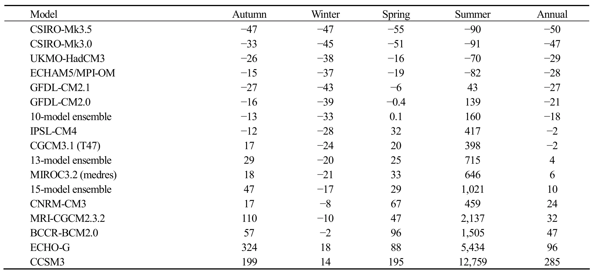
Table 3 Difference percentage of seasonal and annual snow water equivalent between CMIP3 models and remote sensing data during 1979-2000 (unit: %)

Spatial distribution of DPS was further analyzed and Figure 3 shows the situation in winter. Generally, negative differences occupied most areas of Eurasia, but the ranges of positive DPS were greater for most examined models. The distribution of DPS well embodied the geographical features of Eurasia. In the Central Siberian Plateau, all models undervalued SWE with a maximum of about -80%. Under-estimation also existed in the West Siberian Plain from east of the Ural Mountains to west of the Central Siberian Plateau with slightly smaller DPS. However, models exhibited over-estimation in the highlands and plateau region in western China with DPS maxima of about 1,000%. Discrepancies of DPS location mainly existed in the East European Plain. Models such as BCCR-BCM2.0, CGCM3.1(T47), CNRM-CM3, ECHO-G, IPSL-CM4,MRI-CGCM2.3.2, and UKMO-HadCM3 mainly exhibited positive DPS, and the others exhibited mainly negative DPS.As seen from the multi-model ensemble results, the greater positive DPS in the North Siberian Lowland was corrected after abandoning the two models with coarser spatial resolutions. As a result, for Eurasia as a whole, the magnitude of negative DPS in winter increased from -17% to -20%, and the positive DPS in other seasons all decreased to some extent. In annual scale, the DPS decreased from 10% to 4%(Table 3).

4.1.3 Standard deviation of biases

In addition to differences between model and RS data,standard deviation of bias series (SDB) was further computed to examine the consistency of variations for simulations and observations,i.e., the ability of models in simulating the variability of SWE. The spatial distribution of SDB in winter is shown in Figure 4. Clearly, all models simulated better SWE in the Central Siberian Plateau with SDB generally less than 20%. The SDBs were generally 20%-40% in the West Siberian Plain and 60%-100% in Western Europe.

Figure 3 Difference percentage of winter mean snow water equivalent between CMIP3 models and remote sensing data during 1979-2000

The regions with the greatest SDB were the QTP and parts of the East European Plain. The distribution characteristics of SDB indicates where there is greater DPS, there is greater SDB, disclosing worse simulation on variability corresponding to greater differences in magnitude spatially. For Eurasia as a whole, the ascending order for the multi-year mean SDB for annual SWE was CSIRO-Mk3.5,CSIRO-Mk3.0, UKMO-HadCM3, ECHAM5/MPI-OM,10-model ensemble, CGCM3.1 (T47), GFDL-CM2.1,IPSL-CM4, GFDL-CM2.0, MIROC3.2 (medres), 13-model ensemble, CNRM-CM3, 15-model ensemble,BCCR-BCM2.0, CCSM3, MRI-CGCM2.3.2, and ECHO-G.Discounting the greater SDB on the QTP for all models, the reason for ECHO-G, MRI-CGCM2.3.2, BCCR-BCM2.0,and CNRM-CM3 all exhibiting greater SDB is that they simulated worse variability of SWE in Western Europe than other models. For CCSM3, as mentioned before, the SDB in annual scale was inevitably greater due to fewer grids with valid SWE caused by its value assignment principle. However, the SDB for CCSM3 in winter was comparable to those for other models. If eliminating the counteraction of positive and negative biases when calculating mean DPS,i.e., using the absolute values of biases instead, the spatial pattern in winter and the sequencing in annual values of absolute DPS were both the same as those of SDB. This indicates that models whose simulations were of greater biases usually cannot catch the variations of SWE well. As far as the multi-model ensemble results, SDB for annual SWE decreased from 2,460% to 1,822%, and the abnormal large values of SDB in the North Siberian Lowland in winter also decreased to some extent (Figure 4). Based on the analyses above, models of ECHO-G, CCSM3, BCCR-BCM2.0,and MRI-CGCM2.3.2 were screened out for not attending aggregation due to relative weak spatial correlation with and great departures from RS data. Compared to 14-model ensemble results, SWE from the 10-model ensemble was much closer to RS data. First, the simulated abnormal large values on the QTP were corrected (Figure 1), and the spatial correlation coefficients with RS data were improved distinctly, especially in winter (Figure 2). For annual SWE, the spatial correlation coefficient increased from 0.40 to 0.65,and improved from 0.27, 0.49, and 0.55 to 0.74, 0.63, and 0.65 in autumn, winter, and spring, respectively (Table 2).For DPS, the over-estimations were distinctly reduced (Table 3), especially on the QTP (Figure 3). Additionally, the SDB decreased from 1,822% to 699% indicating the improvement of simulating ability in SWE variability, and increased improvement occurred in the region with larger SDB,e.g., the QTP and parts of Europe (Figure 4). Therefore, after examination and elimination, multi-model ensemble results were better at describing distribution and variations of Eurasian SWE. The following projection of Eurasian SWE in the next 50 years was performed based on the 10-model ensemble results.

Figure 4 Standard deviation of relative biases between winter mean snow water equivalent from CMIP3 models and remote sensing during 1979-2000

4.2. SWE in the next 50 years projected by the selected CMIP3 models

Based on the aforementioned examinations, ten of 14 models were selected for arithmetic integration to analyze the changes of Eurasian SWE during 2002-2060. The selected models include CGCM3.1 (T47), CNRM-CM3,CSIRO-Mk3.0, CSIRO-Mk3.5, ECHAM5/MPI-OM,GFDL-CM2.1, GFDL-CM2.0, IPSL-CM4, MIROC3.2(medres), and UKMO-HadCM3.

4.2.1 Temporal and spatial trends

Considering the differences in snow amount between seasons, both absolute and relative trends were examined.The seasonal and annual trends of SWE under SRES A2 and B1 during 2002-2060 are listed in Table 4. Over Eurasia as a whole, the SWE presents a significant (p＜0.05) decreasing trend in both seasonal and annual scale, disclosing a significant decrease of Eurasian SWE in the near future. The decreasing rates under SRES A2 are generally greater than those under SRES B1, irrespective of absolute or relative trends in both seasonal and annual scale, representing a more rapid reduction of SWE when employing a higher GHG emission scenario. The absolute trends for annual SWE under SRES A2 and B1 are -0.33mm/10yrs and-0.30mm/10yrs, respectively, and the relative trends are-1.2%/10yrs and -1.1%/10yrs. The emission of GHG will quicken the reduction of Eurasian SWE. Therefore, controlling GHG emissions will be favorable to the mitigation of Eurasian SWE reduction or disappearance. Additionally, the declining rate for relative trends is the fastest/slowest in summer/winter when snow is the least/most and temperature is the highest/lowest indicating that SWE is more sensitive in warmer versus colder seasons. However, the magnitude of the decrease is not the greatest in winter when the SWE is the most; it is found that magnitude of decrease is the most in spring. This is possibly related to the coexistence of both negative and positive spatial trends. Spatial distribution of absolute trends was further examined.

Table 4 Trends of seasonal and annual snow water equivalent under SRES A2 and B1 during 2002-2060 (p＜0.05)

Figure 5 shows the absolute trends for annual and seasonal SWE in the period of 2002-2060. In annual scale,SWE presents increasing characteristics in northeastern Eurasia and decreasing in other regions, with greater negative trends occurring in both Western Europe and the QTP.Also, the extent and intensity are both greater under SRES A2 than those under SRES B1. The maximum positive and negative trends are 1.4 mm/10yrs and -5.5 mm/10yrs under SRES A2, respectively, and 0.9 mm/10yrs and -5.8 mm/10yrs under SRES B1, respectively. This indicates that different GHG emission scenarios will not only affect the extent of increasing or decreasing SWE, but also distinctly affect increasing amplitude more than decreasing amplitude.Seasonally, there are both significant decreasing trends in autumn and summer, but the amplitudes are all relatively small except for those on the QTP. Meanwhile, SWE also exhibits significant increasing trends in northeastern Eurasia in winter and spring. In winter, the maximum positive and negative trends are 2.9 mm/10yrs and -5.0 mm/10yrs under SRES A2, respectively, and are 1.8 mm/10yrs and -4.9 mm/10yrs under SRES B1, respectively. In spring, they are 2.8 mm/10yrs and -7.4 mm/10yrs under SRES A2, respectively, and 2.4 mm/10yrs and -7.2 mm/10yrs under SRES B1, respectively. Additionally, as seen from Figure 5, the negative trends are generally greater in Europe in spring than in winter, but the extent of positive trends in northeastern Eurasia in spring is not as large as that in winter. The characteristics of greater declining rate and less increasing rate in spring than in winter lead to the overall decreasing trend being greater in spring than in winter for Eurasia as a whole (Table 4). Moreover, the features of increasing in the northeastern and decreasing in other regions are more obvious under SRES A2 than B1.

The aforementioned analyses disclose that, on the one hand, high emission of GHG will quicken the disappearance of snow cover over Eurasia, especially in the West European Plain and the QTP; on the other hand, increasing SWE in the Central Siberian Highlands may be of greater intensity due to increased water vapor caused by global warming. Briefly,if performing higher GHG emission scenario, the SWE for Eurasia as a whole will decrease quicker, and the characteristics of increasing in northeastern Eurasia and decreasing in northwestern Eurasia and the QTP will be clearer. However,irrelevant of performing higher or lower GHG emissions scenarios, the changing patterns of SWE over Eurasia, including the QTP, are not favorable for increasing precipitation in the middle and lower reaches of the Yangtze River in the next 50 years (Chen and Yan, 1979, 1981), but both favor the rain belt moving northward in summer (Wuet al.,2009), just to different extents. It seems that the policy for GHG emission will not be detrimental to the summer rain belt position, but will determine the degree of SWE reduction, which in turn significantly affects Eurasian water resources and the ecosystem.

4.2.2 Relative changes in the middle of 21st century

Taking the mean over the years 2041-2060 to represent the situation in the middle of the 21st century, the spatial distributions of DPS between 2041-2060 and 1971-2000 under SRES A2 and B1 were further examined to quantify the proportion of decreasing SWE (Figure 6). There were similarities in the SWE changes in the middle of the 21st century under higher and lower GHG emission scenarios.The SWE increases in the northeastern Eurasia and decreases in the other regions, and the magnitude of increase is less than that of decreases. The maxima of increasing and decreasing for DPS located in northeastern and southwestern Eurasia, respectively. The increases of annual mean SWE are generally within 10% for both scenarios, with parts of regions increasing 10%-20% under SRES A2. Meanwhile,the magnitude of decrease goes up southward, and above-80% in the south of Western Europe and the QTP. Seasonally, the decrease is found to be the greatest in summer with region-wide consistent change of SWE, although only northeastern Eurasia and the QTP are covered by snow. In autumn, snow-covered area extents, and SWE decreases are almost everywhere, from around 10% in northeastern Eurasia to above 80% in the south edge of Eurasia, except for an increase of less than 10% in the northernmost part of northeastern Eurasia in the middle of 21st century. In winter and spring, the decreases maintain but the area with increased SWE expands to most of northeastern Eurasia with more distinct increase in intensity and extent in winter than in spring. Moreover, differences are also found for the changes under the two scenarios. The decrease and increase under SRES A2 are both greater than those under SRES B1, irrelevant of annual or seasonal scale. Generally, SWE increases less than 10% under SRES B1 in winter and spring,while the increasing percentage goes above 10% in large areas of northeastern Eurasia. This indicates that more emissions of GHG will quicken the decrease of SWE in southwestern and southern Eurasia, and at the same time favor an increase of SWE in northeastern Eurasia.

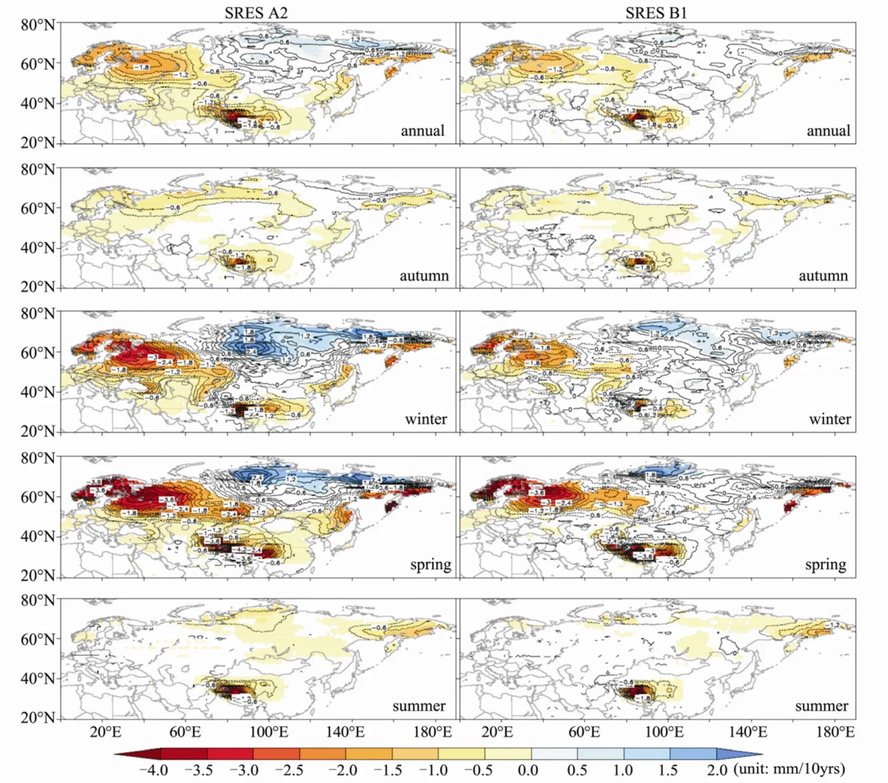
Figure 5 Spatial distribution of trends for annual and seasonal snow water equivalent from aggregated CMIP3 models during 2002-2060.Grey solid line denotes country boundaries, and black solid and dashed lines denote positive and negative trends, respectively.The shaded areas are regions with trends reaching 95% significant level.

5. Conclusion and discussion

Based on run1 from 14 of the 24 CMIP3 models, this paper first validated the ability of each model to simulate the SWE over Eurasia. This was carried out by comparing the output of the models in 20C3M with space-based observa-tions from SMMR and SSM/I in the period from 1979 to 2000. The methods for assessment include computing the relative biases and the spatial correlation coefficient between SWE from models and RS, and the standard deviation of bias series. Then, the SWE from 10 of the 14 models that presented closer relationship and smaller biases with RS data (i.e., CGCM3.1 (T47), CNRM-CM3,CSIRO-Mk3.0, CSIRO-Mk3.5, ECHAM5/MPI-OM,GFDL-CM2.1, GFDL-CM2.0, IPSL-CM4, MIROC3.2(medres), and UKMO-HadCM3) are aggregated into an ensemble average during the period from September 2001 to August 2060. Variations of the projected SWE are investigated under SRES A2 and B1 both temporally and spatially.

Figure 6 Different percentages of aggregated snow water equivalent during 2041-2060 and 1971-2000 for SRES A2 and B1 in annual and seasonal scale

Significant (p＜0.05) decreasing trends of SWE are found to dominate Eurasia in the period from 2002 to 2060 under both SRES A2 and B1. Increasing temperature may have played a significant role by reducing the proportion of snowfall to precipitation (Groismanet al., 2005) and increasing snowmelt. In seasonal scale, the relative trends of decreasing SWE will be the greatest in summer when the air temperature is the highest and the snow cover is the least,which indicates that snow cover in warmer season is more sensitive to climate warming. Increasing air temperature, on the one hand, provides less accumulation of snowfall; on the other hand, accelerates the speed of snow melt (Räisänen,2008; Maet al., 2011). However, the absolute trends of decreasing SWE will not be the greatest in winter when air temperature is the lowest and snow cover is the most, but in spring instead. This is caused by distinct decrease of SWE in western Eurasia and less distinct increase of SWE in northeastern Eurasia in spring than in winter.

Additionally, the extent and rate of decrease for Eurasian SWE are both greater under SRES A2 than B1. This indicates that higher GHG emissions will be detrimental for maintaining snow cover and accelerate the rate of decline.Therefore, it is important to control the emission of GHG for the existence of Eurasian snow cover. Meanwhile, the in-creasing trends differ from each other under different GHG emission scenarios, with greater increases under SRES A2 than B1. The increasing SWE in northeastern Eurasia may be related to increasing winter precipitation (Groismanet al.,2004; Christensenet al., 2007). Projected by IPCC AR4,precipitation in northern Eurasia will distinctly increase,even more than 50%, under moderate GHG emission scenario (SRES A1B) at the end of the 21st century (Christensenet al., 2007). However, winter is the season with steady snow cover in northeastern Eurasia. As a result, increased precipitation will hardly reflect the increase of snow cover area, but instead the amount of snow cover. This kind of characteristics will be more remarkable under higher GHG emission scenario.

分析师称，目前国内花生市场略有涨跌两难的情况，一方面，是农户惜售，各主产区花生上货量较小；另一方面，市场当前消耗有限，经销商采购较为消极；而内贸市场整体库存较为充足，销量不快，多是以质论价。从花生压榨的内在动力来看，市场依然后劲不足。究其原因是花生压榨的下游产品价格不振，花生油市场需求继续平淡，而花生粕价格均有下跌，压榨风险加大，需求也较为疲弱，因此，花生压榨利润难以提高，这对于花生收购积极性也产生一定的影响。截止到目前，国内大型油厂依然没有入市收购，而入市收购的油厂收购较为严格，收购好货为主，采购意愿不强，多固定客户送货或内部自行采购以及竞标采购为主。

Furthermore, there is a basic consensus that Eurasian snow cover in the former winter and spring plays an important role in the summer rain belt in eastern China through its impact on summer monsoon. For Eurasian SWE, an overall decrease is favorable for increase rainfall in southern and southeastern China in summer, and the characteristics of increasing in northeastern Eurasia and decreasing in western Eurasia which favor increased rainfall in North China(Zhanget al., 2008; Wuet al., 2009). Moreover, less snow cover over the QTP is not favorable for summer rainfall in the middle and lower reaches of the Yangtze River (Zhanget al., 2004; Zhao and Moore, 2004). Therefore, the projecting results of Eurasian SWE in this paper favor the summer rain belt moving northward in China, and higher GHG emission will speed up this process. However, the impact of SWE over Eurasia or the QTP on the summer climate in China is not independent. Factors like the ENSO, NAO, and blocking high also play important roles in the relationship between SWE and the succeeding climate. Therefore, changes of summer rain belt in China cannot be determined by any single factor including Eurasian SWE. Moreover, distinct variations including increase and decrease under SRES A2 than B1, irrelevant of seasonal or annual scale, reflect that higher GHG emissions will be more favorable for increase SWE in eastern Eurasia and decrease in western Eurasia,hence more favorable for summer precipitation in North China, but not in the middle and lower reaches of the Yangtze River (Wuet al., 2009). However, in the current climate situation, it is necessary for the relationship between snow cover and summer rain belt in China to be discussed further.Changes of the rain belt are also determined by the impact of climate warming on atmospheric circulation, such as the westerlies, monsoons, and the ocean.

Although the conclusions put forward in this paper are reliable due to its scientific research process, the accuracy of projection will be undoubtedly enhanced if the following problems are solved. Firstly, accuracy of the released RS SWE data will be enhanced if it can be corrected by numerous ground-based observations (Armstronget al., 2007).Secondly, simulations are limited by their poor ability to reproduce SWE in less snow-covered and mountainous areas, such as the south edge of Eurasia and the QTP. More

attention should be paid when discussing the SWE variations in these areas. The discovered increase or decrease in SWE is determined by balancing snowmelt and proportion of snowfall to precipitation caused by increasing air temperature and precipitation. It is trickier in less snow-covered areas or in warmer regions. Local factors such as topography,aspect, vegetation, and blowing snow transport have been shown to further complicate the climate response of SWE in mountainous regions (Brown and Mote, 2009). Thirdly,there are, to some extent, uncertainties in projection performance in a regional scale by using global model results(Gaoet al., 2001). Introducing regional climate model with higher resolution will greatly enhance the accuracy of climate projection (Gaoet al., 2003; Songet al., 2008; Shiet al., 2010). Finally, the ensemble method applied in this study is based on the arithmetic mean, which considers the model results in equal weighting. Development of a suitable ensemble method may improve the accuracy of the resulting projections.

This study was in part supported by the National Natural Science Foundation of China (40901045). We acknowledge the modeling groups, PCMDI and WGCM for their roles in making available the WCRP CMIP3 multi-model dataset.Support of this dataset is provided by the Office of Science,U.S. Department of Energy.

ACIA, 2004. Arctic Climate Impact Assessment (ACIA): Impacts of a Warming Arctic. Cambridge University Press, NY, New York, pp. 144.DOI: 10.2277/ 0521617782.

Armstrong RL, Brodzik MJ, 2002. Northern Hemisphere EASE-Grid weekly snow cover and sea ice extent version 2. National Snow and Ice Data Center, Boulder CO, USA.

Armstrong RL, Brodzik MJ, Knowles K, Savoie M, 2007. Global monthly EASE-Grid snow water equivalent climatology. National Snow and Ice Data Center, Boulder CO, USA.

Brown RD, Mote PW, 2009. The response of Northern Hemisphere snow cover to a changing climate. Journal of Climate, 22(8): 2124-2145. DOI:10.1175/2008JCLI2665.1.

Chang ATC, Foster JL, Hall DK, 1987. Nimbus-7 SMMR derived global snow cover parameters. Annals of Glaciology, 9: 39-44.

Chen LT, Yan ZX, 1979. Influences of snow cover over the Tibetan Plateau during winter and spring on atmospheric circulation and on rainfall over the southern China in pre-monsoon period. In: Collected Papers on Long-term Hydrologic and Meteorological Forecasts (I). Water Conservancy and Power Press, Beijing, pp. 185-194.

Chen LT, Yan ZX, 1981. Statistical analyses on impacts of snow cover over the Tibetan Plateau during winter and spring on the pre-monsoon.In: Collected Papers on Long-term Hydrologic and Meteorological Forecasts (II). Water Conservancy and Power Press, Beijing, pp.133-141.

Christensen JH, Hewitson B, Busuioc A, Chen A, Gao X, Held I, Jones R,Kolli RK, Kwon WT, Laprise R, Magaña Rueda V, Mearns L, Menéndez CG, Räisänen J, Rinke A, Sarr A, Whetton P, 2007. Regional Climate Projections. Climate Change 2007: The Physical Science Basis.Contribution of Working Group I to the Fourth Assessment Report of the Intergovernmental Panel on Climate Change. In: Solomon S, Qin DH,Manning M, Chen ZL, Marquis M, Averyt KB, Tignor M, Miller HL(eds.). Cambridge University Press, Cambridge, United Kingdom and New York, NY, USA.

Ding YH, Ren GY, Zhao ZC, Xu Y, Luo Y, Li QP, Zhang J, 2007. Detec-tion, attribution and projection of climate change over China. Desert and Oasis Meteorology, 1(1): 1-10.

Gao XJ, Zhao ZC, Ding YH, 2003. Climate change due to greenhouse effects in Northwest China as simulated by a regional climate model.Journal of Glaciology and Geocryology, 25(2): 165-169.

Gao XJ, Zhao ZC, Ding YH, Huang RH, Giorgi F, 2001. Climate change due to greenhouse effects in China as simulated by a regional climate model. Advances in Atmospheric Sciences, 18(6): 1224-1230.

Groisman PY, Knight RW, Easterling DR, Hegerl GC, Razuvaev VN, 2005.Trends in intense precipitation in the climate record. Journal of Climate,18 (9): 1326-1350. DOI: 10.1175/JCLI3339.1.

Groisman PY, Knight RW, Karl TR, Easterling DR, Sun B, Lawrimore JH,2004. Contemporary changes of the hydrological cycle over the contiguous United States: Trends derived from in situ observations. Journal of Hydrometeorology, 5(1): 64-85. DOI: 10.1175/1525-7541(2004)005＜0064:CCOTHC＞2.0.CO;2.

Hosaka M, Nohara D, Kitoh A, 2005. Changes in snow coverage and snow water equivalent due to global warming simulated by a 20km-mesh global atmospheric model. Scientific Online Letters on the Atmosphere,1: 93-96. DOI: 10.2151/sola.2005-025.

Lemke P, Ren JW, Alley RB, Allison I, Carrasco J, Flato G, Fujii Y, Kaser G, Mote P, Thomas RH, Zhang T, 2007. Observations: Changes in Snow,Ice and Frozen Ground. Climate Change 2007: The Physical Science Basis. Contribution of Working Group I to the Fourth Assessment Report of the Intergovernmental Panel on Climate Change. In: Solomon S,Qin DH, Manning M, Chen ZL, Marquis M, Averyt KB, Tignor M,Miller HL (eds.). Cambridge University Press, Cambridge, United Kingdom and New York, NY, USA.

Ma LJ, Qin DH, Bian LG, Xiao CD, Luo Y, 2011. Assessment of snow cover vulnerability over the Qinghai-Tibetan Plateau. Advances in Climate Change Research, 2(2): 93-100. DOI: 10.3724/SP.J.1248.2011.00093.

Meehl GA, Stocker TF, Collins WD, Friedlingstein P, Gaye AT, Gregory JM, Kitoh A, Knutti R, Murphy JM, Noda A, Raper SCB, Watterson IG,Weaver AJ, Zhao ZC, 2007. Global Climate Projections, in Climate Change 2007: The Physical Science Basis. 100. In: Solomon S, Qin DH,Manning M, Chen ZL, Marquis M, Averyt KB, Tignor M, Miller HL(eds.). Cambridge University Press, Cambridge, United Kingdom and New York, NY, USA.

Meleshko VP, Kattsov VM, Govorkova VA, Malevsky-Malevich SP, Nadyozhina ED, Sporyshev PV, 2004. Anthropogenic climate changes in the 21st century in Northern Eurasia. Russian Meteorology and Hydrology, 7: 5-26.

Murakami H, Wang B, 2010. Future change of North Atlantic tropical cyclone tracks: projection by a 20-km-mesh global atmospheric model. J.Climate, 23(10): 2699-2721. DOI: 10.1175/2010JCLI3338.1.

PaiMazumder D, Miller J, Li Z, Walsh JE, Etringer A, McCreight J, Zhang T,Molders N, 2007. Evaluation of Community Climate System Model soil temperatures using observations from Russia. Theoretical and Applied Climatology, 94(3-4): 187-213. DOI: 10.1007/s00704-007-0350-0.

Räisänen J, 2008. Warmer climate: less or more snow? Climate Dynamics,30(2-3): 307-319. DOI: 10.1007/s00382-007-0289-y.

Shepard D, 1968. A Two-Dimensional Interpolation Function for Irregularly-Spaced Data. The 1968 ACM National Conference, Harvard College, Cambridge, Massachusetts.

Shi Y, Gao XJ, Wu J, Filippo G, Dong WJ, 2010. Simulation of the changes in snow cover over China under global warming by a high resolution RCM. Journal of Glaciology and Geocryology, 32(2): 215-222.

Shi YF, 2001. Estimation of the water resources affected by climatic warming and glacier shrinkage before 2050 in West China. Journal of Glaciolgy and Geocryology, 23(4): 333-341.

Shi YF, Liu SY, 2000. Projection of glaciers in China responding to the global warming in the twenty-first century. Chinese Science Bulletin,45(4): 434-438.

Song RY, Gao XJ, Shi Y, Zhang DF, Zhang XW, 2008. Simulation of changes in cold events in southern China under global warming. Advances in Climate Change Research, 4(6): 352-356.

Wu BY, Yang K, Zhang RH, 2009. Eurasian snow cover variability and its association with summer rainfall in China. Advances in Atmospheric Sciences, 26(1): 31-44. DOI: 10.1007/s00376-009-0031-2.

Xu Y, Ding YH, Li DL, 2003a. Climatic change over Qinghai and Xizang in 21st century. Plateau Meteorology, 22(5): 451-457.

Xu Y, Ding YH, Zhao ZC, 2003b. Scenario of temperature and precipitation changes in Northwest China due to human activity in the 21st century.Journal of Glaciolgy and Geocryology, 25(3): 327-330.

Xu Y, Ding YH, Zhao ZC, 2004. Prediction of climate change in middle and lower reaches of the Yangtze River in the 21st century. Journal of Natural Disasters, 13(1): 25-31.

Xu Y, Ding YH, Zhao ZC, Zhang J, 2003c. A scenario of seasonal climate change of the 21st century in Northwest China. Climatic and Environmental Research, 8(1): 19-25.

Zhang RH, Wu BY, Zhao P, Han JP, 2008. The decadal shift of the summer climate in the late 1980s over eastern China and its possible causes. Acta Meteorologica Sinica, 22(4): 435-445.

Zhang YS, Li T, Wang B, 2004. Decadal change of the spring snow depth over the Tibetan Plateau: The associated circulation and influence on the East Asian summer monsoon. Journal of Climate, 17(14): 2780-2793.DOI: 10.1175/1520-0442(2004)017＜2780:DCOTSS＞2.0.CO;2.

Zhao HX, Moore GWK, 2004. On the relationship between Tibetan snow cover, the Tibetan Plateau monsoon and the Indian summer monsoon. Geophysical Research Letters, 31: L14204. DOI: 10.1029/2004GL020040.

Zhao ZC, Ding YH, Xu Y, Zhang J, 2003. Detection and prediction of climate change for the 20th and 21st century due to human activity in Northwest China. Climatic and Environmental Research, 8(1): 26-34.

Zhao ZC, Luo Y, Gao XJ, Xu Y, 2007a. Projections of typhoon changes over the western North Pacific Ocean for the 21st century. Advances in Climate Change Research, 3(3): 158-161.

Zhao ZC, Luo Y, Jiang Y, Xu Y, 2008. Assessment and prediction of precipitation and droughts/floods changes over the world and in China. Science & Technology Review, 26(6): 28-33.

Zhao ZC, Wang SW, Luo Y, 2007b. Assessments and projections of temperature rising since the establishment of IPCC. Advances in Climate Change Research, 3(3): 183-184.

10.3724/SP.J.1226.2012.00093

*Correspondence to: Dr. LiJuan Ma, Associate Research Fellow of the National Climate Center, China Meteorological Administration.No. 46, Zhongguancun Nandajie, Haidian District, Beijing 100081, China. Tel: +86-10-68406544; Email: malj@cma.gov.cn

August 12, 2011 Accepted: November 3, 2011