Simulation of water entry of an elastic wedge using the FDS scheme and HCIB method*

Simulation of water entry of an elastic wedge using the FDS scheme and HCIB method*

SHIN Sangmook, BAE Sung Yong

Department of Naval Architecture and Marine Systems Engineering, Pukyong National University, Busan 608-737, Korea, E-mail: smshin@pknu.ac.kr

(Received August 10, 2012, Revised October 30, 2012)

The hydroelasticity of water entry of an elastic wedge is simulated using a code developed using the flux-difference splitting scheme for immiscible and incompressible fluids and the hybrid Cartesian/immersed boundary method. The free surface is regarded as a moving contact discontinuity and is captured without any additional treatment along the interface. Immersed boundary nodes are distributed inside a fluid domain based on the edges that cross an instantaneous body boundary. Dependent variables are reconstructed at each immersed boundary node with the help of an interpolation along a local normal line for providing a boundary condition for a discretized flow problem. A dynamic beam equation is used for modeling the elastic deformation of a wedge. The developed code is validated through comparisons with other experimental and computational results for a free-falling wedge. The effects of the elastic deformation of the wedge on the pressure fields and time histories of the impact force are investigated in relation to the stiffness and density of the structure. Grid independence test is carried out for the computed time history of the force acting on an elastic wedge.

hydroelasticity, free surface capturing, non-boundary conforming method, dynamic beam equation, free falling, impact force

Introduction

The dynamic interactions between free surface flows and elastic structures are common in various engineering problems, including the slamming of a ship or the sloshing of liquid in a cargo tank. Recently, many researchers have reported experimental or computational results on hydroelasticity. Luo et al.[1]combined the Wagner theory and the finite element method to analyze the slamming problem and reported that flexible rigidity has effects on high-frequency oscillations in the stresses. Korobkin et al.[2]analyzed water entry of an elastic structure using the Wagner theory and the added masses of elastic plates. Peseux et al.[3]carried out experiments on the free fall droptests of rigid and elastic cones and reported the limitation of the Wagner theory, which are related to the jet phenomena. Hua et al.[4]used the arbitrary Lagrange-Euler fluid-field model and simulated the water ditching of an airplane. Panciroli et al.[5]used the smoothed particle hydrodynamics to estimate the hydrodynamic impact during the water entry of an elastic wedge. Das and Batra[6]used a coupled Lagrangian and Eulerian formulation to analyze the slamming and reported that the deformation of a structure has significant effects on the pressure distribution on a body. Although various methods have been suggested for analyzing hydroelasticity, the deforming boundary around a fluid still poses challenging problems for numerical schemes.

Non-boundary conforming methods, including the immersed boundary method, offer advantages in the handling of deforming boundaries because these methods use simple background grids, whose boundaries do not conform to the boundaries of instantaneous fluid domains. Gilmanov and Sotiropoulos[7]suggested the Hybrid Cartesian/Immersed Boundary (HCIB) method. In contrast to the immersed boundary method, a computational domain is defined as a subset of an instantaneous fluid domain, which enables the HCIB method to easily handle infinitesimally thin bodies and inviscid flows. Shin et al.[8]suggested a criterionbased on the edges crossing a body boundary to guarantee that a discretized flow problem is well posed in the HCIB method. Shin et al.[9]combined the HCIB method and a dynamic beam equation to simulate the increased propulsive efficiency of a heaving foil caused by the flexibility of the foil.

Many methods for simulating free surface flows have been suggested, including the volume of fluid method, the level set method, and the ghost fluid method. However, these methods require additional treatments along an interface, such as the construction of an instantaneous free surface and enforcement of the dynamic condition of a free surface. These additional treatments may cause difficulties in the accurate conservation of each fluid component or in the construction of accurate interfaces as an interface undergoes complicated changes. Recently, a free surface capturing method[10,11]has been developed, where an interface is regarded as a moving contact discontinuity. The free surface capturing method was expanded on the basis of the Flux-Difference Splitting (FDS) scheme for variable density incompressible fluids.

Shin et al.[12]suggested a new method based on the FDS scheme for variable density incompressible fluids and the HCIB method to simulate free surface flows around moving or deforming bodies. The developed FDS-HCIB code was thoroughly validated through comparisons with other experimental and computational results on various free surface flows, including water waves generated by a hydrofoil, a moving wave-maker, and emerging or sinking cylinders near interfaces. The FDS-HCIB code was also applied to simulate the generation of a tsunami caused by a deforming bed and violent three-dimensional sloshing in a spherical tank. In this study, the FDS-HCIB code is expanded to simulate hydroelasticity by augmenting the dynamic beam equation. To validate the developed code, which is combined with an equation of body motion, the free fall of a rigid wedge is simulated and the computed results are compared with other experimental and computational results. Finally, the code is applied to simulate the hydroelasticity of water entry of an elastic wedge.

1. Mathematical modeling and numerical methods

The governing equations are the conservation of mass and momentum, and the incompressibility condition of each fluid. A material interface is captured as a moving contact discontinuity in a flow field. To allow for this discontinuity within a fluid domain, the governing equations are written in the form of the integral conservation law as follows:

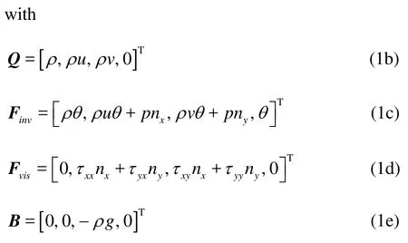
whereΩis the control volume,Sis the control surface,ρis the density,uandv are the respective x- andy -velocities,p is the pressure,nxand nyare the unit normal vector components,θis the normal velocity with respect to the control surface,τijis the shear stress tensor, andg is the gravitational acceleration.

The FDS scheme[12]for variable density incompressible fluids is used for calculating numerical inviscid fluxes across discontinuities in a fluid domain. For each physical time step, a hyperbolic system of a Riemann problem is formulated by introducing artificial compressibility with respect to the pseudo-time as follows:

whereβis the artificial compressibility parameter with respect to the pseudo-timeτ. For Eq.(2a), the original conservation laws are recovered as a steady state solution is obtained with respect to the pseudotime. Based on a solution of the Riemann problem, the numerical flux can be written as

The HCIB method[8]is used to enforce the boundary condition for a dynamically deforming body. A Cartesian background grid is used to discretize the governing equations. To define the boundary of an instantaneous computational domain, Immersed Boundary (IB) nodes are distributed within a fluid domain so that the computational domain is a subset of the fluid domain. The set of IB nodes should appropriately represent a body boundary, regardless of the body configuration. In addition, the set of IB nodes should define a closed computational domain so that the discretized flow problem is well-posed by the boundary conditions described at the IB nodes. To meet these requirements, IB nodes are identified based on the edges crossing a body boundary[8]. Using this criterion, a node is identified as an IB node whenever an interior node is connected to an edge crossing a body boundary. For each physical time step, a deforming body boundary is defined by a set of line segments connecting two neighboring Lagrangian points on a body boundary. Velocity vectors are given at those Lagrangian points as the body boundary condition of the original flow problem. To identify the IB nodes, it is checked whether each edge of the background grid makes contact with any line segment on the body boundary.

For each identified IB node, a local normal line that passes through the given IB node and orthogonally intersects a body boundary is assigned. For each local normal line, a velocity vector is interpolated at the point of intersection on the body boundary by using the velocity vectors described at two neighboring Lagrangian points. The local normal line is extended into a fluid domain, and the other endpoint is located on an edge of a background grid. Dependent variables are interpolated at this endpoint by using dependent variables at two nodes of the edge of the background grid. The interpolated dependent variables are updated within one physical time step as the pseudo-time iteration progresses for satisfying the condition of incompressibility.

To estimate the dependent variables at each IB node, dependent variables are reconstructed along the local normal line by using interpolated dependent variables at both endpoints. For the velocity vector, a linear variation along the local normal line is assumed near the given IB node. The density is extrapolated from a fluid domain. The dynamic pressure is extrapolated from a fluid domain, and the pressure is then corrected on the basis of the hydrostatic pressure gradient.

2. Flow over a flexible plate

To validate the developed FDS-HCIB code for the interaction between an elastic body and flow, flow over a flexible plate is simulated using the present code. For this example, Shin et al.[8]reported their computational results. The same parameters are given to compare two results. The elastic deformation caused by the uniform inflow is modeled based on the dynamic beam equation as follows[8,13]

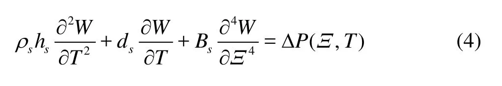
whereΞis the coordinate along a surface of the plate without deformation,W( Ξ, T)is the deformation of the structure,ρsis the density of the structure,hsis the thickness of the structure,dsis the material damping of the structure,Bsis the flexural rigidity of the structure, and ΔPis the pressure difference between two sides of the plate. In this study, the material damping is ignored so thatds=0. Equation (4) can be non-dimensionalized on the basis of the length of the plateLp, the density of fluidρ, and the inflow velocityU∞, as follows:

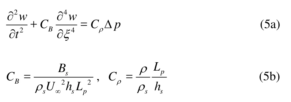
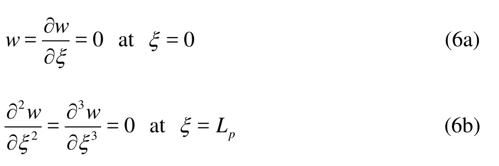
For the boundary condition of the structural deformation, the clamped and free ends conditions are given as follows:

For each physical time step, the distribution of pressure along the plate is calculated, and then Eq.(5a) is solved using the finite difference method to estimate the distribution of the structural deformation. Based on the time variation of the structural deformation, the velocity distribution, which is caused by the structural deformation, is determined.

From the rest, the inflow is accelerated linearly until U∞t/ Lp=2. The plate is released to deform according to the pressure difference between both sides of the plate fromU∞t/ Lp=2. The Reynolds number,U∞Lp/v, is 500 and two parameters CBandCρare given as 0.1. Figure 1 shows computed deformation of the plate and instantaneous vorticity field at U∞t/ Lp=5. In Fig.2, the computed time history of the deformation at thetip is compared with reported results by Shin et al.[8].Good agreementsare achieved for two computational results.

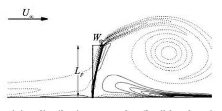
Fig.1 Vorticity distribution around a flexible plate in uniform flow, at U∞t/ Lp=5

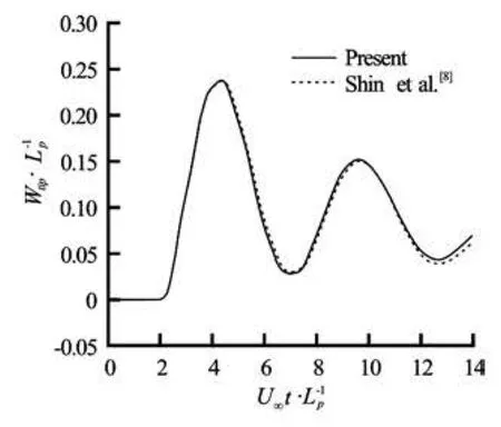
Fig.2 Comparison of time histories of the tip deflection of a flexible plate in uniform flow

Fig.3 Schematic diagram of a free-falling rigid wedge

3. Free fall of a rigid wedge

To validate the developed FDS-HCIB code for the interaction between free surface flow and body motion, the free fall of a rigid wedge was simulated. Zhao et al.[14]carried out experiments that addressed this same problem, and Kleefsman et al.[15]and Oger et al.[16]reported their numerical results by using the volume of fluid method and the Smoothed Particles Hydrodynamics (SPH) method, respectively. Figure 3 shows a schematic diagram of this problem. The width of the wedge,Lw, is 0.5 m and the dead-rise angle,θw, is 30o. Although two-dimensional computations were reported in their numerical simulations, Zhao et al.[14]positioned the measurement section of a 0.2 m length between two dummy sections so that the total length was 1 m. The total mass of the wedge and the drop mechanism,Mw, is 241 kg. The initial entry velocity of the wedge,Vo, is 6.15 m/s, and the entry velocity, V( t), decreases according to the time variation of the force acting on the wedge.

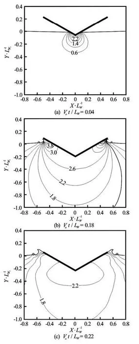
Fig.4 Contours of pressure change,ΔP/0.5ρV2, around a0 free-falling rigid wedge atVot/ Lw=0.04, 0.18, and 0.22

The computational domain is -30 ＜ x/Lw＜30 and -30 ＜ y/Lw＜20, and the minimum grid size is given as0.005Lwaround the wedge. The non-dimensional physical time step size,ΔtVo/Lw, is fixed as 0.002. On the surface of the wedge, 100 Lagrangianpoints are uniformly distributed. The time variation of the entry velocity,V( t ), and the location of the wedge, Y( t), are computed based on Newton’s second law as follows:

Figure 4 shows the time variation of the pressure difference,ΔP, which is the difference between the local pressure and the atmospheric pressure. The pressure difference is non-dimensionalized on the basis of the initial velocity,Vo. At Vot/Lw=0.04, the maximum pressure is exerted near the keel of the wedge, and the pressure decreases monotonically along the surface of the wedge. As water entry progresses, the maximum pressure moves toward near the spray root, which results in rapid pressure changes

near the interface. At Vot/Lw=0.22, the spray root leaves the tip of the wedge and the maximum pressure is again exerted near the keel of the wedge, and the pressure changes quickly diminish. These observations of the pressure fields are in accordance with the results previously reported by Zhao et al.[14]and Oger et al.[16]. In Fig.5, the pressure field at Vot/Lw=0.18 is shown for the case in which the wedge enters the water at a constant speed,Vo. In this case, the pressure changes are greater owing to the absence of deceleration caused by the impact force. However, the pressure field shows characteristics similar to those of the previous case of free fall.

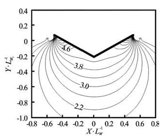
Fig.5 Contours of pressure change,ΔP/0.5ρV2, at V t/ L=0ow 0.18, where a wedge undergoes water entry at a constant speed Vo

In Fig 6, the lower plots show the computed pressure coefficient distribution,Cp= ΔP/0.5ρV( t)2,on the surface of the wedge atVot/Lw=0.18. In this figure, the pressure change is non-dimensionalized on the basis of the instantaneous velocity,V( t). It can be seen that the maximum pressure coefficients are similar if the pressure change is non-dimensionalized on Oger et al.[16]areshown together att=0.0158 s. It this basis. In theupper plot of Fig.6, the distribution of the pressure coefficients reported by Zhao et al.[14]and can be seenthat thepresent resultsare simicomputational resultsreported by Oger et al.[16],whichla rto the were obtained using the SPH method.

Fig.6 Comparisons of distribution of pressure coefficient, C= ΔP/0.5ρV( t)2, on the surface of a wedgep

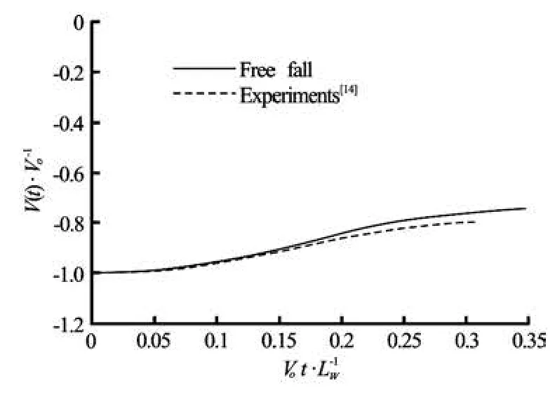
Fig.7 Comparison of time histories of water-entry speed of a free-falling wedge

Figure 7 shows a comparison of the computed time variation of the entry speed,V( t), and the experimental results reported by Zhao et al.[14]. As water entry progresses, deceleration increases untilVot/ Lw=0.18, after which the deceleration decreases as the water impact decreases. Although the present results predict a slightly stronger deceleration, the two results show good agreement. Figure 8 shows the time variation of the vertical force,Fy, acting on the wedge. To estimate the vertical force,Fy, the pressure diffe-rences ΔPand shear stresses are extrapolated at the Lagrangian points. These pressure differences and shear stresses are integrated over the wedge surface on the basis of the normal vectors of line segments connecting neighboring Lagrangian points. Although the present results and the SPH results obtained by Oger et al.[16]overestimate the vertical force, all the results for the case of free fall show a similar time variation of the impact force, which includes a linear increase during the initial phase and an abrupt decrease after the maximum force occurs.

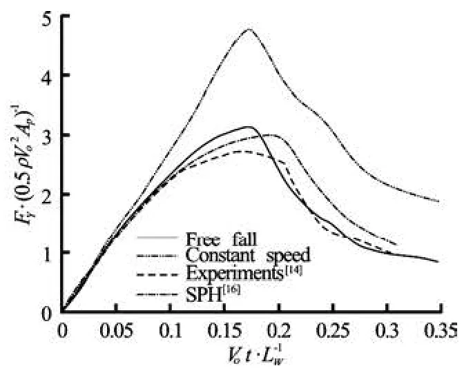
Fig.8 Comparison of time histories of vertical force acting on a water-entry wedge

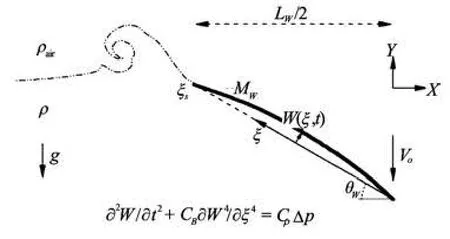
Fig.9 Schematic diagram of water entry of an elastic wedge

4. Water entry of an elastic wedge

The developed FDS-HCIB code was applied to the simulation of the water entry of an elastic wedge at a constant speed,Vo. Figure 9 shows a schematic diagram of this problem. The deformation caused by the time variance of the water impact is modeled based on the dynamic beam equation as was explained in the previous section. In Eq.(5a),ξis the coordinate along a surface of the wedge without deformation and Δpis the difference between pressure on the wedge surface and the atmospheric pressure. For the non-dimensional parameters, the width of the wedge,Lw, the density of water,ρ, and the water entry velocity, V0, are used. For the boundary condition of the structural deformation, it is assumed that each surface of the wedge is simply supported at the center and at both endpoints, as follows

As was pointed out by Shin et al.[9], the structural response is dominated by its low-order eigenmodes, regardless of complicated fluid loads, owing to the filtering effects of the structure itself. This implies that a converged solution of Eq.(5a) can be obtained using a small number of structural elements. For the purpose of computational efficiency, the discretization of the structural elements should be independent of the distribution of the Lagrangian points in the flow computations. To estimate the distribution of the fluid load, the pressure values are extrapolated at the Lagrangian points, and those pressures are then integrated over each structural element. It has been observed that if the total number of structural elements is greater than 20, there is virtually no change in the computed results. Based on the estimated velocity distribution along the structural elements, the velocity vector caused by the structural deformation is interpolated at each Lagrangian point. To provide a boundary condition for the flow problem at the next physical time step, the position and velocity vectors at each Lagrangian point are adjusted by including the effects of water entry velocity,Vo.

Except for the instantaneous entry velocity,V( t), which in this case is fixed as the initial velocity, all the other parameters are the same as those in the previous free-fall case. For the non-dimensional parameters in the dynamic beam equation, the computational results are presented by using two sets of parameters. In the first case, the structure is assumed to be soft and heavy, so that CB=0.01,Cρ=1. In the second case, the non-dimensional parameters are changed to be CB=2,Cρ=20, which corresponds to a hard, light structure.

Figures 10 and 11 show the time evolution of the pressure fields and structural deformations for those two cases. The pressure fields around a rigid wedge that undergoes the same body motion are shown together on the right-hand side of each figure. In Figs.12 and 13, the time variations of the structural deformations are magnified. For the soft heavy structure, it can be seen that the deformation is concentrated near the keel during the initial phase and that the deformation increases monotonically. However, in the case of the hard light structure, the deformation is dominated by the first eigenmode from the initial phase, and vibration occurs as water entry progresses. This difference in the structural deformation results in significant changes in the pressure fields. With the soft heavy structure, the monotonic upward deformation of the structure induces upward suction of neighboring fluid and results in a significant decrease in the pressure changecaused by the downward motion of the wedge’s entry into the water. A similar decrease in pressure change occurs during the initial phase for the hard light structure because of the upward deformation. However, the downward deformation caused by the strong restoring force of flexural rigidity increases the pressure change around the wedge as the water entry progresses. Considering the short time duration of the water entry, the effects of the acceleration of the deformation, i.e., the added mass effect, may dominate the difference in the pressure changes.

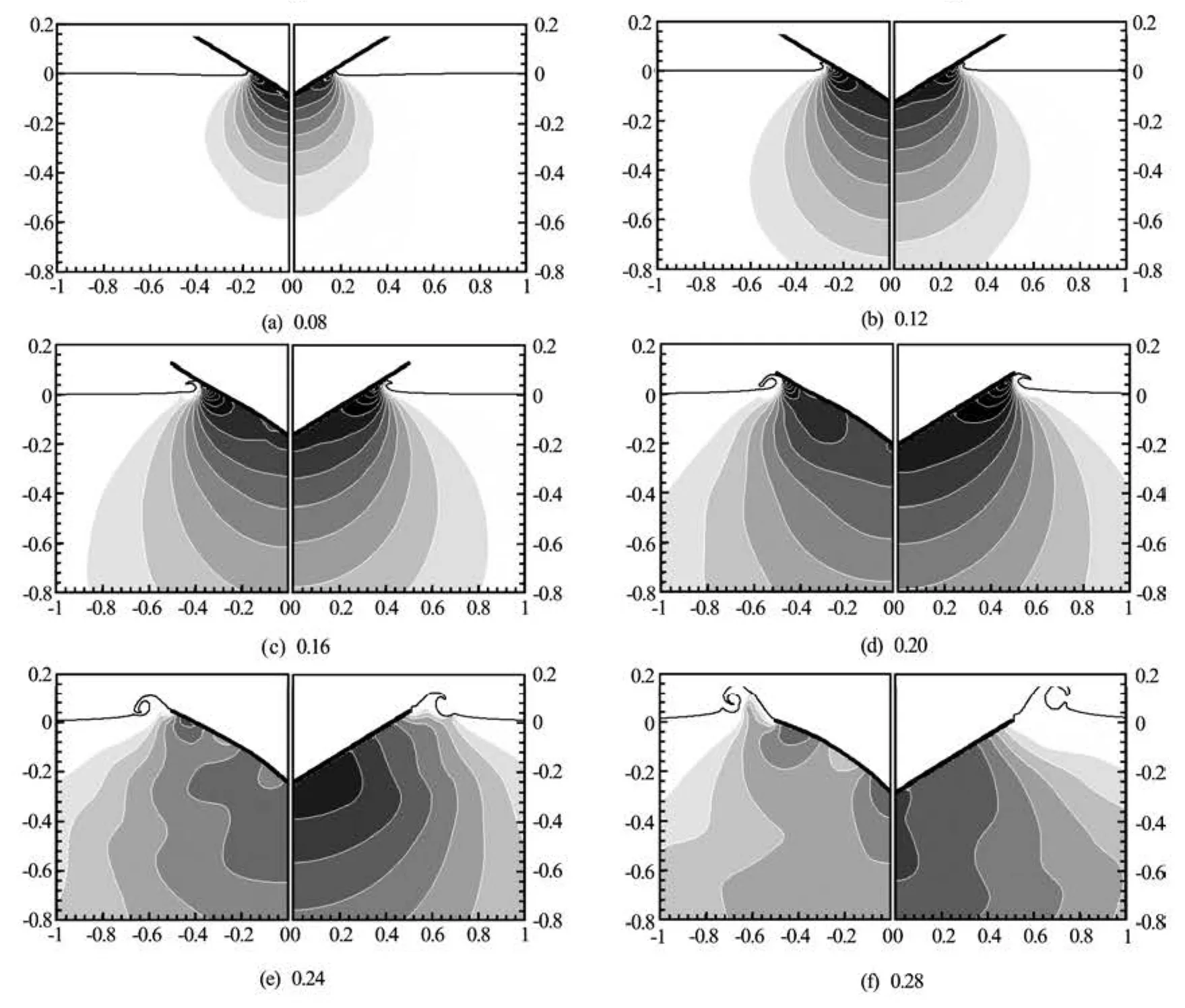
Fig.10 Time evolution of pressure fields around elastic (left) and rigid (right) wedges:CB=0.01,Cρ=1,0.2 ＜Cp＜6.2,ΔCp= 0.4

The difference in the pressure fields results in contrasting changes in the time history of the water impact force. In Fig.14, these changes are compared for the two elastic wedges and a rigid wedge with the same body motion. Compared with the case of the rigid wedge, the impact forces decrease in the initial phase for both elastic wedges. However, for the hard light structure, the impact force increases as the structure undergoes downward deformation. From Figs.13 and 14, it can be observed that the increased impact force caused by the deformation occurs before the deformation reaches its maximum. This observation supports the previous prediction that the added mass effect would be the main cause of the difference in impact force because the downward acceleration of the structural deformation begins to develop before the deformation reaches its maximum.

Grid independence test was carried out for the computed time history of the force acting on the elastic wedge. For fine, medium, and coarse grids, the minimum grid spacing was varied as 0.005Lw,0.01Lwand 0.02Lw, respectively. Figure 15 shows a comparison of the computed time histories of the force, where CBand Cρare given as 0.01 and 1, respectively. Although the results for the coarse grid predicts a smaller degree of fluctuation afterVot/Lw=0.22, the results for fine and medium grids show virtually no difference in the computed time history of the force acting on the elastic wedge. As was mentioned previously, the filtering effects of the structure make it easier to obtain a converged solution for the structural deformation, as compared with a converged solutionfor the flow field around the deforming wedge.

Fig.11 Time evolution of pressure fields around elastic (left) and rigid (right) wedges:CB=2,Cρ=20,0.2＜Cp＜6.2,ΔCp=0.4

5. Conclusions

In this study, a developed code that employs the FDS scheme for variable density incompressible fluids and the HCIB method has been successfully expanded to simulate the hydroelasticity of water entry of an elastic wedge. The use of the FDS scheme and the HCIB method makes it possible to handle the interaction between free surface flows and deforming boundaries automatically, once the position and velocity vectors of the Lagrangian points are provided.

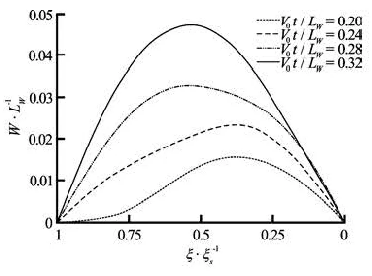
Fig.12 Time variation of computed deflection of an elastic wedge:CB=0.01,Cρ=1

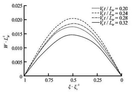
Fig.13 Time variation of computed deflection of an elastic wedge:CB=2,Cρ=20

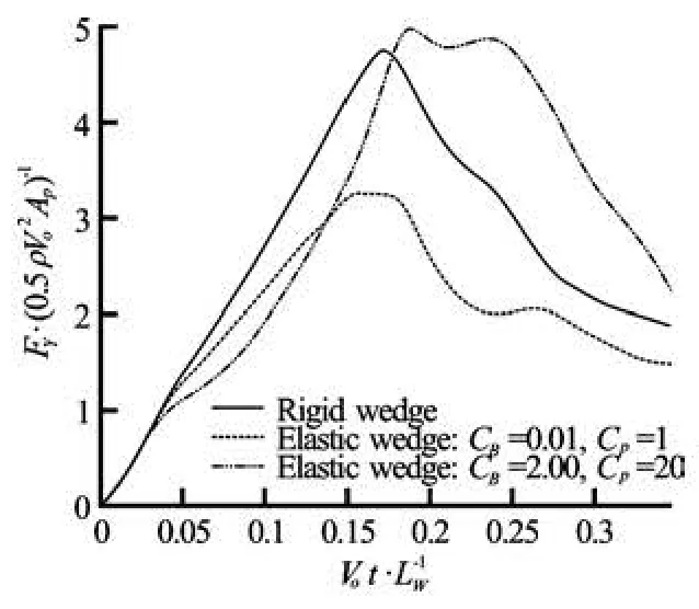
Fig.14 Comparison of time histories of force acting on elastic and rigid wedges

The FDS-HCIB code has been validated for an interaction between a free surface flow and a freely moving body. Good agreement is observed between the present results and other experimental and computational results for the time histories of the velocity and the impact force acting on a free-falling rigid wedge.

In addition, it is observed that the water impact force may increase or decrease according to the flexural rigidity and density of a structure. For the soft heavy structure, the monotonic increase in the deformation causes the upward acceleration of neighboring fluid and results in decrease in the impact pressure.However, for the hard light structure, the downward deformation caused by the vibration results in the stronger impact pressure. Grid independence has been established for the computed time history of the force acting on the elastic wedge, using three different size grids.

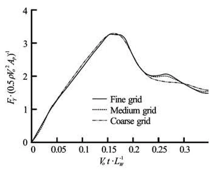
Fig.15 Grid independence test for computed time history of force acting on an elastic wedge:CB=0.01,Cρ=1

Acknowledgement

This work was supported by the Research Grant of Pukyong National University (2013).

[1] LUO H., WANG H. and SOARES C. G. Numerical and experimental study of hydrodynamic impact and elastic response of one free-drop wedge with stiffened panels[J]. Ocean Engineering, 2012, 40: 1-14.

[2] KOROBKIN A., GUERET R. and MALENICA S. Hydroelastic coupling of beam finite element model with Wagner theory of water impact[J]. Journal of Fluids and Structures, 2006, 22(4): 493-504.

[3] PESEUX B., GORNET L. and DONGUY B. Hydrodynamic impact: Numerical and experimental investigations[J]. Journal of Fluids and Structures, 2005, 21(3): 277-303.

[4] HUA Cheng, FANG Chao and CHENG Jin. Simulation of fluid-solid interaction on water ditching of an airplane by ALE method[J]. Journal of Hydrodynamics, 2011, 23(5): 637-642.

[5] PANCIROLI R., ABRATE S. and MINAK G. et al. Hydroelasticity in water-entry problems: Comparison between experimental and SPH results[J]. Composite Structures, 2012, 94(2): 532-539.

[6] DAS K., BATRA C. Local water slamming impact on sandwich composite hulls[J]. Journal of Fluids and Structures, 2011, 27(4): 523-551.

[7] GILMANOV A., SOTIROPOULOS F. A hybrid Cartesian/immersed boundary method for simulating flows with 3D, geometrically complex, moving bodies[J]. Journal of Computational Physics, 2005, 207(2): 457-492.

[8] SHIN S., BAE S. Y. and KIM I. C. et al. Computation of flow over a flexible plate using the hybrid Cartesian/immersed boundary method[J]. International Journal for Numerical Methods in Fluids, 2007, 55(3): 263-282.

[9] SHIN S., BAE S. Y. and KIM I. C. et al. Effects of flexibility on propulsive force acting on a heaving foil[J]. Ocean Engineering, 2009, 36(3-4): 285-294.

[10] QIAN L., CAUSON D. M. and MINGHAM C. G. et al. A free-surface capturing method for two fluid flows with moving bodies[J]. Proceeding of the Royal Society A, 2006, 462(2065): 21-42.

[11] GAO F., INGRAM D. M. and CAUSON D. M. et al. The development of a Cartesian cut cell method for incompressible viscous flow[J]. International Journal for Numerical Methods in Fluids, 2007, 54(9): 1033- 1053.

[12] SHIN S., BAE S. Y. and KIM I. C. et al. Simulation of free surface flows using the flux-difference splitting scheme on the hybrid Cartesian/immersed boundary method[J]. International Journal for Numerical Methods in Fluids, 2012, 68(3): 360-376.

[13] PAN Ding-yi, LIU Hua and SHAO Xue-ming. Studies on the oscillation behavior of a flexible plate in the wake of a D-cylinder[J]. Journal of Hydrodynamics, 2010, 22(5Suppl.): 132-137.

[14] ZHAO R., FALTINSEN O. and AARSNES J. Water entry of arbitrary two-dimensional sections with and without flow separation[C]. 21st Symposium on Naval Hydrodynamics. Trondheim, Norway, 1997, 408-423.

[15] KLEEFSMAN K. M. T., FEKKEN G. and VELDMAN A. E. P. et al. A volume-of fluid based simulation method for wave impact problems[J]. Journal of Com- putational Physics, 2005, 206(1): 363-393.

[16] OGER G., DORING M.and ALESSANDRINI B. et al. Two-dimensional SPH simulation of wedge water entry[J]. Journal of Computational Physics, 2006, 313(2): 803-822.

10.1016/S1001-6058(11)60384-4

* Biography: SHIN Sangmook (1967-), Male, Ph. D., Associate Professor