
Ship bow waves*
2013-06-01 12:29NOBLESSEFrancis
水动力学研究与进展 B辑 2013年4期
NOBLESSE Francis
State Key Laboratory of Ocean Engineering, School of Naval Architecture, Ocean and Civil Engineering, Shanghai Jiao Tong University, Shanghai 200240, China, E-mail: noblfranc@gmail.com
DELHOMMEAU Gerard
Laboratoire de Mecanique des Fluides, Ecole Centrale, Nantes, France
LIU Hua, WAN De-cheng
State Key Laboratory of Ocean Engineering, School of Naval Architecture, Ocean and Civil Engineering, Shanghai Jiao Tong University, Shanghai 200240, China
YANG Chi
School of Physics, Astronomy and Computational Sciences, George Mason University, Fairfax VA, USA
Ship bow waves*
NOBLESSE Francis
State Key Laboratory of Ocean Engineering, School of Naval Architecture, Ocean and Civil Engineering, Shanghai Jiao Tong University, Shanghai 200240, China, E-mail: noblfranc@gmail.com
DELHOMMEAU Gerard
Laboratoire de Mecanique des Fluides, Ecole Centrale, Nantes, France
LIU Hua, WAN De-cheng
State Key Laboratory of Ocean Engineering, School of Naval Architecture, Ocean and Civil Engineering, Shanghai Jiao Tong University, Shanghai 200240, China
YANG Chi
School of Physics, Astronomy and Computational Sciences, George Mason University, Fairfax VA, USA
(Received July 22, 2013, Revised August 1, 2013)
The bow wave generated by a ship hull that advances at constant speed in calm water is considered. The bow wave only depends on the shape of the ship bow (not on the hull geometry aft of the bow wave). This basic property makes it possible to determine the bow waves generated by a canonical family of ship bows defined in terms of relatively few parameters. Fast ships with fine bows generate overturning bow waves that consist of detached thin sheets of water, which are mostly steady until they hit the main free surface and undergo turbulent breaking up and diffusion. However, slow ships with blunt bows create highly unsteady and turbulent breaking bow waves. These two alternative flow regimes are due to a nonlinear constraint related to the Bernoulli relation at the free surface. Recent results about the overturning and breaking bow wave regimes, and the boundary that divides these two basic flow regimes, are reviewed. Questions and conjectures about the energy of breaking ship bow waves, and free-surface effects on flow circulation, are also noted.
bow wave, overturning wave, breaking wave, wave height, wave energy
Introduction
The bow wave generated by a ship hull that advances at constant speed in calm water is considered. While of much lesser practical importance than the drag (of primary importance for design), the sinkage and the trim experienced by a ship, the bow wave is a feature of the flow around a ship hull that is of particular theoretical interest, and worth studying for several reasons. For one, a ship bow wave is a highly visible feature of the flow around a ship hull. Indeed, ship bow waves have been widely studied, experimentally[1-11]as well as numerically or theoretically[12-29].
Furthermore, an important fundamental property of a bow wave is that it only depends on the shape of the ship bow, not the length of the ship or the hull geometry aft of the bow region. This notable feature, which follows from the fundamental property that ship waves do not propagate ahead of a ship, makes it possible to perform systematic parametric studies and to determine the bow waves of a canonical family of ship bows. Indeed, a ship bow can be defined via a relatively small number of parameters (unlike the large number of parameters required to define the geometry of an entire ship hull surface).
Finally, another main property of a ship bow wave is that it is affected by nonlinearities to a far greater extent than the waves aft of the bow wave. Indeed, ship waves, with the notable exception of bow waves, typically are only weakly influenced by nonlinear effects, and in fact can be well approximated as linear waves for most practical purposes. A direct consequence of strong nonlinear effects at a ship bow is that ship bow waves can be divided into two distinctflow regimes. Specifically, fast ships with fine bows generate overturning bow waves that consist of detached thin sheets of water, which are mostly steady until they hit the water and undergo turbulent breaking up and diffusion. However, slow ships with blunt bows create highly unsteady and turbulent breaking bow waves. The boundary between the steady overturning bow wave regime and the unsteady turbulent breaking bow wave regime readily follows from an upper bound for the elevation of the free surface that is a direct consequence of the nonlinear Bernoulli relation for steady free surface flows. Ship bow waves therefore provide a rich test case for investigating the influence of flow nonlinearities associated with the boundary condition at the free surface, and for testing the capabilities of CFD methods. Breaking ship bow waves may also be interesting more broadly to investigate the energy contained in breaking waves.
The article reviews recent results related to the overturning and breaking bow wave regimes, and the boundary that divides these two flow regimes. Questions and conjectures about the energy of breaking ship bow waves, and free-surface effects on flow circulation, are also noted. The article mostly focuses on analytical approximations, based on elementary considerations and experimental measurements or observations. This emphasis is justified by the fact that analytical approximations are necessary to gain basic insight into the complex nonlinear dynamics of ship bow waves, notably the existence of two alternative flow regimes and the prediction of the boundary between these flow regimes, and are useful for many practical purposes.
1. A basic nonlinear constraint
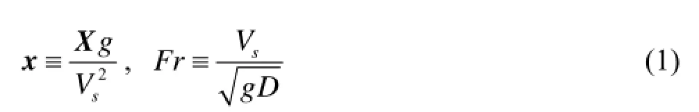
We then consider the bow wave created by a ship hull, with draft D, that steadily advances at speed Vsalong a straight path in calm water of effectively infinite depth and lateral extent. The flow around the ship hull is observed from a right handed moving system of orthogonal coordinates X≡(X,Y,Z )attached to the ship, and thus appears steady with flow velocity given by the sum of an apparent uniform current (Vs,0,0) opposing the ship speed Vsand the (disturbance) flow velocity U≡(U,V,W)due to the ship. The X axis is chosen along the path of the ship and points toward the ship stern. The Z axis is vertical and points upward, with the mean (undisturbed) free surface taken as the plane Z=0. We define the nondimensional coordinates x and the draft-based Froude number Fr as
The elevation of the free surface is denoted E. Viscous and surface tension effects are ignored. For steady flows, the Bernoulli relation

therefore holds. Here P is the flow pressure, Patm.is the atmospheric pressure, and ρ is the density of water. At the free surface, where Z=E and P=Patm., the Bernoulli relation becomes
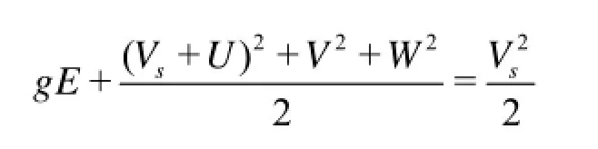
This relation yields the (well-known) upper bound

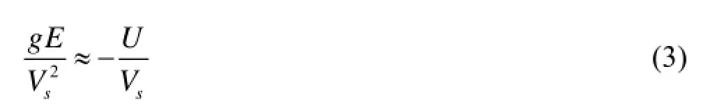
for the free-surface elevation E for steady free-surface flows. This upper bound is a direct and important consequence of the nonlinear Bernoulli relation. If the nonlinear terms in the Bernoulli relation are neglected, the upper bound (2) does not hold and the Bernoulli relation yields the (well-known) linearized approximation
The highest free-surface elevationbZ for a ship bow wave occurs at the crest of the bow wave. Thinship theory and experimental measurements show that the bow wave height bZ is roughly proportional to the entrance angle α of the waterline at the ship stem. If we consider a family of ship bows with various waterline entrance angles α, we readily anticipate that the“steady-flow constraint” (2) is satisfied for values of α that are sufficiently small, but cannot be satisfied for large values of α. Thus, steady bow waves can be expected for fine ship bows. However, steady bow waves cannot exist for blunt ship bows. The nonlinear constraint (2) therefore implies two types of bow waves that correspond to two distinct flow regimes. Specifically, fast ships with fine bows generate overturning bow waves that consist of detached thin sheets of water, which are mostly steady until they hit the water and undergo turbulent breaking up and diffusion. However, slow ships with blunt bows create highly unsteady and turbulent breaking bow waves. Furthermore, the conditiondetermines the boundary between the “steady” overturning bow wave regime and the unsteady turbulent breaking bow wave regime. Thus, the existence of two distinct bow wave regimes, and the boundary that divides these two alternative flow regimes, immediately follow from an elementary consideration of the Bernoulli relation. The steady overturning and breaking bow wave regimes, and the related dividing boundary, are successively considered below.

The linear approximation (3) allows waves of large amplitude and cannot predict the occurrence of wave-breaking. While this property implies important limitations of a linearized theory of free-surface flows, the fact that a linear theory can predict large waves without wavebreaking is actually quite useful for many practical applications. Furthermore, the excess wave energy radiated by the overly large waves that can be predicted by a linear theory approximately accounts for the energy that would be dissipated via wavebreaking within a nonlinear theory, as shown in Ref.[30]. For the practical numerical modeling of flows around ship hulls, linear theories are therefore advantageous, indeed are arguably much preferable to nonlinear theories, in many instances. However, a nonlinear theory is necessary to gain a realistic understanding of ship bow waves.
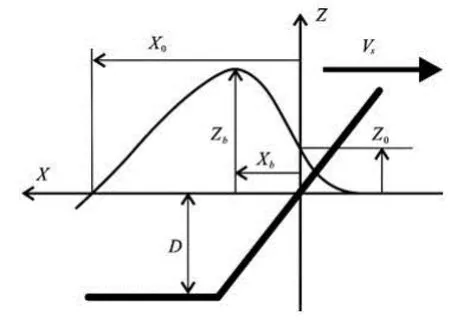
Fig.1 Ship draft D and speed sV, rise of water 0Z at the ship stem, bow wave heightbZ, distancebX between the ship stem and the bow wave crest, and distance0X between the ship stem and the crossing of the bow wave with the mean free-surface plane =Z0
2. Overturning bow waves
2.1 Analytical bow wave profiles for fine ship bows with rake and flare
As depicted in Fig.1, a bow wave profile (contact curve between a ship hull surface and the free surface) is largely determined by four basic features: the height Zbof the bow wave (elevation of the bow wave crest above the mean free-surface plane Z=0), the location Xb(measured from the ship stem X=0) of the bow wave crest, the water height Z0at the ship stem X= 0, and the length X0of the bow wave (specifically, X0defines the location, measured from the ship stem, of the intersection of the bow wave profile with the mean free-surface plane Z=0).
The front face of a bow wave (bow wave front) is well approximated by a parabolic arc, as suggested in Ref.[25] and experimentally verified in Ref.[11]. The back face can also be (crudely) approximated by a parabolic arc. Thus, the front and back faces of a bow wave can be approximated by the two parabolic arcs

Here ζ is used instead of z to emphasize that the foregoing expressions define the wave profile z= ζ(x). Furthermore, xsin (5a) corresponds to the intersection x=xsof the bow wave profile with the ship stem line x=-ztan β. The intersection xsand the corresponding water elevation zsare given by
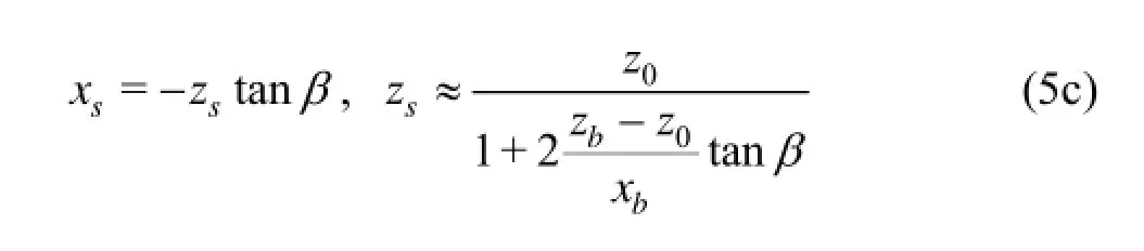
The relation for zsis based on an approximation in which, within the short segment xs≤x<0, the parabolic arc (5a) is replaced by its tangent at x=0.
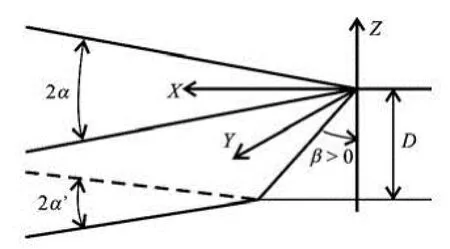
Fig.2 Four-parameter (draft D, rake angle β, and entrance angles 2α and 2α′ of top and bottom waterlines) family of ship bows with rake and flare
Simple analytical approximations to the four basic flow features bZ, bX, 0Z and 0X are given in Refs.[23-25] for a (particularly simple) family of wedge-shaped ship bows defined by only two parameters (the waterline entrance angle 2α and the draft D) and in Refs.[26,27] for the more general family ofship bows depicted in Fig.2. This family of ship bows is defined by four parameters: the draft D, the rake angle β, and the hull entrance angles 2α and 2α′ at the top waterline (at the free surface =0Z) and at the bottom waterline (at the hull draft =ZD-), respectively. The wedge-shaped bows considered in Refs.[23-25] correspond to the special case =0β and =αα′.
The analysis (based on dimensional analysis, experimental measurements, elementary asymptotic considerations, and extensive applications of thin-ship theory) given in Refs.[23-27] yields the simple analytical relations
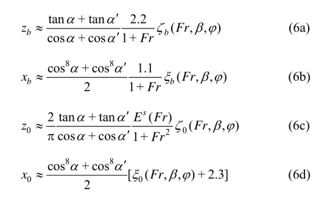
where φ is related to the flare of the bow and is defined in terms of the waterline angles α and α′ as

Fr is the draft-based Froude number (1) and the function Es(Fr) is defined in Ref.[27].
The four functions ζb(Fr,β,φ), ξb(Fr ,β,φ), ξ0(Fr ,β,φ) and ξ0(Fr,β,φ) are tabulated in Ref.[27] for six draft-based Froude numbers Fr that correspond to Fr/(1+Fr)=0.3, 0.4, …, 0.8, nine rake angles β=60o, 45o, …, -60o, and nine values of the hull flare parameter φ=1, 0.75, …, -1. These ranges of Froude numbers, rake angles, and flare en- compass most cases of practical interest. In particular, the range 0.3≤Fr/(1+Fr)≤0.8 corresponds to draft- based Froude numbers Fr in the range 0.43≤Fr≤4 and-for a ship with length/draft ratio Ls/D=20-to length-based Froude numbersin the range 0.1≤FrL≤0.9.
The relations (6) yield useful physical insight into main characteristics of ship bow waves. In particular, we have

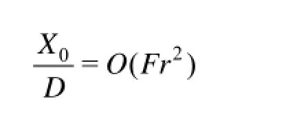
in the high-speed limit Fr→∞. Here, (1) was used.
Expressions (5) and (6) provide simple analytical approximations to the bow wave profiles of a relatively broad class of fine ship bows with rake and flare. The effect of a bulb can be approximately taken into account by adding the wave profile due to a point source.
2.2 Experimental and CFD validation
The simple analytical approximations (6) to the four basic featuresbZ,bX,0Z and 0X that largely characterize a ship bow wave profile are compared to experimental measurements for wedge-shaped ship bows with various entrance angles 2α, and also for a rectangular flat plate towed at several yaw (incidence) angles α, in Refs.[23-25]. The wedge-shaped bows correspond to the special case =0β and =αα′ of the ship bows depicted in Fig.2.

Fig.3 Normalized bow wave height (Zbg/Vs2)cosα/tan α for ten hull forms (top), and a rectangular flat plate towed at three yaw angles α, several speeds Vsand heel angles γ (bottom). The straight solid line is the approximation 2.2/(1+Fr) given by (7), and the dashed curve corresponds to Ogilvie’s high-Froude-number approximation
In particular, expression (6a) for the bow wave heightbZ yields
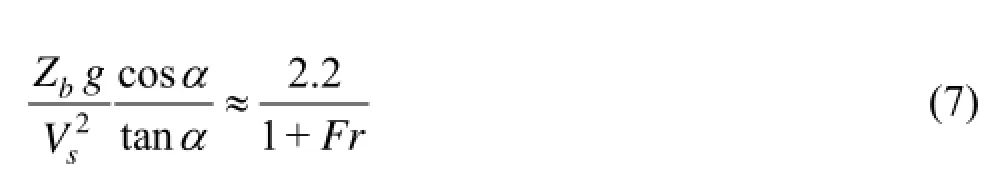
for wedge-shaped bows. The analytical approximation (7) is compared to experimental measurements in Fig.3 for wedge-shaped ship bows with various entrance angles 2α (top) and for a rectangular flat plate towed at several yaw angles α (bottom). The high Froude number approximation proposed by Ogilvie[31]is also shown in Fig.3.
Detailed comparisons of analytical predictions and experimental measurements ofbX,0Z and0X for both wedge-shaped ship bows with various entrance angles and a rectangular flat plate at several yaw angles are also given in Refs.[23-25]. Furthermore, comparisons of experimental wave profiles with the analytical wave profiles predicted by (5) and (6) are given in Ref.[25] for wedge-shaped ship bows (Wigley hull and three sharp-ended strut-like hulls) with various entrance angles as well as a rectangular flat plate at several yaw angles.
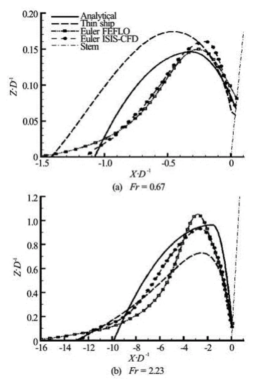
Fig.4 Analytical wave profile given by (5) and (6) and wave profiles obtained from thin-ship theory and two CFD flow solvers (ISIS-CFD and FEFLO), used in Euler-flow mode, for the ship bow shown in Fig.2 with β=30oand α′=α=15o, at two draft-based Froude numbers Fr= 0.67 and 2.23. The stem line of the ship is marked in the figure
For the more general family of ship bows depicted in Fig.2, the analytical bow wave profile given by the two parabolic arcs (5) and the relations (6) is shown in Ref.[27] to be in good overall agreement with CFD bow wave profiles obtained via Euler-flow calculation methods. This result is illustrated in Fig.4 where the analytical wave profile given by (5) and (6) is compared to wave profiles obtained from two CFD flow solvers (ISIS-CFD and FEFLO) used in Eulerflow mode, as well as thin-ship theory, for the ship bow shown in Fig.2 with =β30oand ==αα′15o, at two draft-based Froude numbers =Fr0.67 and 2.23.
The Euler profiles in Fig.4 are appreciably closer to the parabolic bow-wave profiles (5) than to the wave profiles given by thin-ship theory, which is used in Refs.[26,27] to extend the relations obtained (using elementary theoretical considerations, notably dimensional analysis, and experimental measurements) in Refs.[23-25] for wedge-shaped bows (without rake or flare) to the more general family of ship bows depicted in Fig.2.
Thus, the simple analytical relations (5) and (6), with the tables for the functions ζb, ξb, ζ0, ξ0given in Ref.[27], provide a practical analytical approximation to the bow wave profile for xs≤x≤x0. This simple approximation may be useful for a relatively broad class of fine bows with rake and flare, common for fast ships that generate overturning bow waves.
2.3 Free-surface effects at the leading edge of a plate
An interesting result of the experimental observations and measurements reported in Ref.[25] is that a rectangular flat plate towed at a yaw angle α creates a bow wave that does not differ appreciably from the bow wave generated by a wedge-shaped bow with entrance angle 2α. This notable property is illustrated in Fig.3, where the bow wave height Zbis depicted for a wedge (top) and for a flat plate (bottom).
The close similarity of 3-D flows about a wedge or the related inclined vertical flat plate (one side of the wedge) in the presence of a free surface is markedly different from the corresponding case of unbounded 2-D flows (i.e., without a free surface) about a wedge (with entrance angle 2α) advancing straight ahead at constant speed or about the flat plate (at an incidence angle α) that is obtained when one side of the wedge is removed.
A possible explanation for this difference is that no flow circulation is generated around the leading edge of a flat plate piercing a free surface because the pressure at the free surface is constant (equal to the atmospheric pressure). Thus, the presence of a free surface may have a large influence on flow circulation. Further experimental and CFD investigations of freesurface effects on flow circulation may then be interesting.
2.4 Elementary theory of overturning bow waves
Overturning ship bow waves cannot be predicted using traditional methods, notably thin-ship theory and potential-flow panel methods, for computing flows around ship hulls. However, divergent overturning bow waves can be predicted and evaluated using the 2-D+t theory as well as numerical (CFD) methods[12-22]. Although modern CFD methods can be used to compute overturning detached ship bow waves, as is indeed illustrated further on, such numerical calculations are not well suited for performing the systematic parametric studies that are required to analyze the influence of a ship’s speed and draft, and of the shape of a ship bow. CFD methods likewise are not well suited for routine practical applications to design, notably at early stages when numerous alternative designs typically need to be considered.
The elementary theory of overturning ship bow waves expounded in Ref.[29] provides a complementary alternative approach to CFD. The fully-analytical, albeit highly-simplified, theory expounded in Ref.[29] yields direct “cause-and-effect” relationships between-on the “cause” side-the ship speedsV and the bow geometry (draft D, entrance angles α and α′ at the top and bottom waterlines, rake angle β and related flare) and-on the “effect” side-main geometrical characteristics (size, shape, thickness) of the resulting detached overturning bow wave and the width of the related wave breaking wake. The theory also provides basic physical insight that is not readily provided by the detailed experimental measurements or CFD calculations reported in the literature on ship bow waves[2,3,20,22], into the relatively complex dynamics of overturning ship bow waves.
The theory ignores effects of viscosity and surface tension. Although this basic approximation greatly simplifies the flow analysis, the inviscid-flow analysis of an overturning ship bow wave remains extremely complex, notably due to strong nonlinearities in the free-surface boundary condition. Additional approximations are therefore made in the elementary theory considered in Ref.[29], although it accounts for nonlinearities as required to model overturning ship bow waves. The theory consists of four main steps.
The first step is the contact curve, commonly called bow wave profile, between the ship hull and the free surface. For the relatively broad class of fine ship bows with rake and flare depicted in Fig.2, this first step can be taken as the analytical approximation to the bow wave profile given by (5) and (6).
In the second step, the flow velocity at the bow wave profile is determined from the bow wave profile-via simple analytical relations-by means of the exact (for an inviscid flow) boundary conditions at the ship hull surface and the free surface, this second step is given in Refs.[32,29].
The third step, expounded in Ref.[29], determines the overturning detached bow wave and the wave’s size, shape, and intersection with the mean free surface. This step is an elementary Lagrangian analysis, based on Newton’s equations, that ignores interactions among water particles within the overturning detached bow wave.
The (unpublished) fourth step determines the thickness of the overturning ship bow wave (thin sheet of water) via elementary considerations related to mass conservation, specifically by relating the volume of water that flows through an overturning bow wave to the water displaced by the advancing ship hull.
These four steps fully determine the size, shape and thickness of an overturning bow wave and the width of the related wavebreaking wake in terms of the ship speed and the bow geometry (draft and shape) for the relatively broad class of fine ship bows depicted in Fig.2. The qualitative comparisons with experimental observations and CFD calculations reported in Ref.[29] show that while the elementary analysis underlying the theory cannot be expected to yield accurate predictions, the theory predicts trends correctly and provides useful estimates of the influence of main ship design parameters (speed, draft, bow shape), for which systematic experimental measurements or CFD computations are not available.
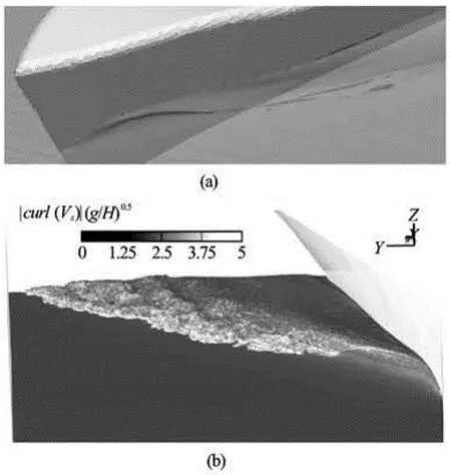
Fig.5 Simulated by the RANS solver FOAM-SJTU[34](a) or the SPH method[35](b)
2.5 CFD simulations of overturning bow waves
The results summarized in the foregoing, and indeed throughout most of this article, largely consider analytical approximations, based on elementary considerations and experimental measurements or observations. As already noted, this focus is justified by the fact that analytical approximations are useful for practical applications, and indeed are necessary to gainbasic insight into the complex nonlinear dynamics of ship bow waves, notably the occurrence of two flow regimes and the approximate prediction of the related dividing boundary.
However, ship bow waves can also be computed using CFD methods, as illustrated in Refs.[22,29,33-35]. Two recent examples of numerical simulations of overturning ship bow waves, reported in Refs.[34] and [35] are shown in Fig.5. The numerical simulations depicted in the upper part of the figure are obtained using the RANS solver naoe-FOAM-SJTU[36-38]. The lower part of Fig.5 shows numerical simulations given by a meshless-based Lagrangian particle method[39-41].
The numerical simulations depicted in Fig.5 and elsewhere[22,29,33], are in qualitative agreement with flow observations, e.g., with the pictures shown in Ref.[25], as well as the elementary analytical theory expounded in Ref.[29]. Quantitative comparisons between detailed experimental measurements and numerical or theoretical predictions of the size, shape and thickness of an overturning bow wave, and of the width of the related wave breaking wake, clearly are needed to better ascertain the merits and the limitations of CFD methods and the elementary analytical theory given in Ref.[29].
3. Boundary between overturning and breaking bow waves
3.1 Theoretical boundary between two types of bow waves
Expression (6a) for the bow wave amplitude zband the upper bound zb≤1/2 for steady free-surface flows show that steady overturning ship bow waves can only exist if
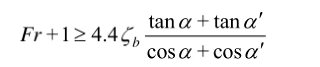
In the special case of wedge-shaped bows, this condition becomes

These conditions are satisfied for fast ships with fine bows, but not for slow ships with blunt bows.
3.2 Experimental validation
For wedge-shaped ship bows, the boundary between the steady overturning bow wave regime and the unsteady breaking bow wave regime is then given by

Experimental validation of this simple analytical approximation for the boundary between the two basic bow wave regimes is considered in Refs.[25] and [28].
For each of the nine yaw angles α, computerdriven color photographs (eight for 10oα≤≤45o, ten for =α75oand 90o, eleven for =α60o) of the bow wave are taken. Figure 6 shows the resulting series of (photographed) instantaneous bow wave profiles for two yaw angles =α15o(a) or 60o(b). As already noted, these two yaw angles correspond to the overturning or breaking bow wave regimes, respectively,according to the theoretical relation (8). There is little variation among the bow wave profiles in the top of Fig.6, i.e., for the yaw angle =α15o. However, considerably more variation can be observed among the bow wave profiles for =α60o, in the bottom of Fig.6.

Fig.6 Instantaneous bow wave profiles (determined from photographs) due to a rectangular flat plate, immersed at a draft D=0.2m , towed at constant speed Vs= 1.75 m/s in calm water, and held at a heel angle 10oand two yaw angles α=15oor 60o, which correspond to the overturning and unsteady bow wave regimes, respectively
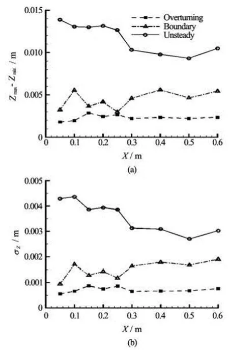
Fig.7 Averages of the variations Zmax-Zmin(top) and σz(bottom) for α=10o, 15o, 20oand for α=30o, 45o, 60o, 75o, 90o. These averages correspond to the overturning and unsteady bow wave regimes, respectively, and are marked “overturning” and “unsteady” in the figure. The third curve, marked “boundary”, corresponds to α=25o, which lies on the boundary (8) between the overturning and unsteady wave regimes
Two alternative quantitative measures of the variations among the bow wave profiles shown in Fig.6 are considered in Fig.7. Specifically, the (top) and (bottom) of Fig.7 show averages of the largest variations Zmax-Zmin(top) or of the root-mean-square variationszσ (bottom), respectively, among bow wave heights at nine values =X0.05 m, 0.1 m, 0.15 m, 0.2 m, 0.25 m, 0.3 m, 0.4 m, 0.5 m and 0.6 m of the distance from the leading edge of the plate. Two curves in Fig.7 correspond to averages for =α10o, 15o, 20oon one hand, and for =α30o, 45o, 60o, 75o, 90oon the other hand. The resulting average values of Zmax-Zminand σzare marked “overturning” and“unsteady” in Fig.7. The line marked “boundary” in Fig.7 corresponds to =α25o, which lies on the boundary (8) between the overturning and unsteady wave regimes.
Figure 7 shows that the largest variation Zmax-Zminand the rms variation σzare significantly larger for 30o≤α≤90othan for 10o≤α≤20o. Thus, Fig.7 shows that bow waves for 30oα≤≤90oexhibit a significantly higher degree of unsteadiness than bow waves for 10oα≤≤20o, especially near the leading edge of the plate, which corresponds to small values of X in Fig.7.
A more detailed study of the difference in flow unsteadiness between the “steady” overturning bow wave regime and the breaking wave regime is given in Ref.[28]. Further experimental illustrations of the change flow regime that occurs at the boundary (8) are given in Ref.[25] where several photographs of bow waves generated by a flat plate are shown. The transition between the two bow wave regimes is also well illustrated in three videos that can be viewed at http://www.scs.gmu.edu/?rlohner/pages/pics/freesurf. html.
4.Breaking bow waves
4.1 Height of breaking bow waves
The heightbZ of a (highly unsteady, turbulent) breaking ship bow wave, that is generated by a “slow”ship with a “blunt” bow as already noted, is now considered. The (top) and (bottom) of Fig.8 depict the normalized bow wave heights Zbg/Vs2and (1+ Fr)Zg/V2, respectively, as functions of the water
bs line half entrance angle α, or for a flat plate the yaw angle α. Figure 8 shows a relatively large number of experimental measurements (for eleven hulls and a flat plate towed at nine yaw angles). The experimental data are divided into two groups, identified by ○ or +, which correspond to values of α and Fr in the unsteady (breaking) or steady (overturning) bow wave regimes. This division into steady and unsteady data is not based on flow observations, but is determined by the values of α and Fr with respect to the theoretical boundary (8).
Figure 8(a) shows that the steady-flow data (+) lie below the horizontal line Zbg/Vs2=1/2, in agreement with the Bernoulli constraint Zbg/Vs2≤1/ 2 for steady free-surface flows. Figure 8(a) also shows that the unsteady-flow data (○) are distributed, more or less evenly, around the horizontal line Zbg/Vs2= 1/2. Thus, the height Zbof an unsteady ship bow wave is given byin accordance with the constraint imposed by the Bernoulli relation for steady free-surface flows.
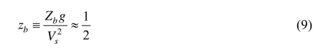
Figure 8(b) shows that the steady-flow data (+) are distributed, fairly evenly, around the curve 2.2tan/cosαα, in agreement with the approximation (7) and Fig.3. Figure 8(b) also shows that the unsteady-flow data (○) are located below the curve 2.2tan/cosαα.

Fig.8 Bow wave heights Zbg/Vs2(top) and (1+Fr)Zbg/Vs2(bottom) as functions of the waterline half entrance angle α or the yaw angle α for a flat plate. The experimental measurements identified by ○ or + correspond to values of α and Fr within the unsteady or steady bow wave regimes
Thus, expressions (7) and (9) provide reasonable approximations to the heightbZ of a ship bow wave in the overturning and unsteady flow regimes. These expressions also provide upper bounds forbZ in the unsteady and overturning regimes, respectively. Indeed, the heightbZ of the bow wave of a ship with a wedge-shaped bow is given by

Figure 8 shows that this simple expression agrees relatively well with experimental measurements for hulls with wedge-shaped bows as well as a flat plate. Expression (10) directly defines the heightbZ of a ship bow wave, that may be overturning or unsteady, in terms of the ship speedsV, draft D, and waterline entrance angle 2α.
4.2 Energy of breaking bow waves
A nonbreaking plane progressive wave is fully defined by a relatively small number of parameters: the angle θ that determines the direction of propagation of the wave, the wave length λ or the related wave number k≡2π/λ, the wave period T or the related wave frequency ω≡2π/T , the water depth H, and the wave amplitude A. Furthermore, the wavenumber k, the wave frequency ω, the water depth H and the wave amplitude A are related via a dispersion relation, where the wave amplitude has no significant influence if A is small enough. E.g., the dispersion relation is k=ω2/g for the simplest case of small waves in deep water.
The energy transported by a nonbreaking plane progressive wave is determined in terms of the wave amplitude as2/2gAρ in deep water. However, the situation is quite different and considerably more complex for breaking waves, including breaking ship bow waves of interest here, because the wave amplitude is no longer a meaningful parameter as noted earlier. Thus, the energy of a breaking ship bow wave, and more generally of other types of breaking water waves, cannot be determined in terms of the wave amplitude A as for the much simpler case of nonbreaking plane progressive waves. Indeed, the determination of the energy of a breaking wave is a nontrivial fundamental issue.
A reasonable conjecture is that this energy can be related to the volume ∇ of the breaking wave, instead of its amplitude A. Indeed, elementary considerations suggest that the kinetic energy and the potential energy of a breaking ship bow wave may be assumed proportional to ρ∇Vs2. The energy of a breaking bow wave can be related to the drag experienced by a ship bow. This relationship may then provide useful information about the energy of breaking ship bow waves. Detailed experimental measurements, as well as numerical computations, of breaking ship bow waves would be very useful, and indeed are necessary to gain a realistic understanding of this important but complex flow regime.
5. Conclusions
In summary, several practical results about the bow wave generated by a ship hull that advances at constant speed in calm water have been reviewed. These results-based on simple considerations, notably dimensional analysis, experimental measurements, elementary asymptotic considerations, and extensiveapplications of thin-ship theory-include simple analytical relations that approximately determine bow wave profiles for the relatively broad class of fine bows with rake and flare depicted in Fig.2. The effect of a bulb can be approximately taken into account by adding the wave profile due to a point source.
A fundamental constraint (upper bound for the free-surface elevation), that stems from the nonlinear Bernoulli relation for steady free-surface flows, implies the existence of two basic alternative bow wave regimes. Specifically, fast ships with fine bows generate overturning bow waves that consist of detached thin sheets of water, which are mostly steady until they hit the main free surface and undergo turbulent breaking up and diffusion. However, slow ships with blunt bows create highly unsteady and turbulent breaking bow waves. The boundary that separates these two flow regimes readily follows from the constraint associated with the Bernoulli relation. For the family of ship bows shown in Fig.2, the boundary between the “steady overturning” and “unsteady breaking”regimes is given by a simple analytical relation.
The simple analytical relations for bow wave profiles, and the boundary that separates the overturning and breaking bow wave regimes, summarized here agree well with experimental observations and measurements for wedge-shaped ship bows with various entrance angles as well as a flat plate towed at various yaw angles. The analytical bow wave profiles are also in fair agreement with CFD computations for the fine ship bows with rake and flare depicted in Fig.2.
The reviewed results also include an elementary fully-analytical, albeit highly-simplified, theory that determines the size, shape and thickness of an overturning bow wave, and the width of the related wave breaking wake, in terms of the ship speed and the bow geometry (draft and shape) for the class of ship bows shown in Fig.2. Qualitative comparisons with experimental observations and CFD calculations show that while this elementary theory cannot be expected to be accurate, it predicts trends correctly and provides useful estimates of the influence of main ship design parameters (speed, draft, bow shape).
Ship bow waves offer a rich test case for investigating the influence of flow nonlinearities associated with the boundary condition at the free surface, and for testing the capabilities of CFD methods. Breaking ship bow waves created by slow ships with blunt bows may also provide useful insight into the basic issue of determining the energy contained in a breaking wave, which cannot be readily evaluated in terms of the wave amplitude as for the much simpler case of a nonbreaking plane progressive wave. A reasonable conjecture is that the energy of a breaking bow wave can be related to the volume ∇ of the breaking wave, instead of its amplitude A, and may be assumed proportional to ρ∇Vs2.
Ship bow waves also illustrate the basic difficulties inherent to the nonlinear modeling of free-surface flows around ship hulls. Indeed, although a linearized theory of free-surface flows has important limitations (including the inability to predict wavebreaking), it allows large waves without the occurrence of wavebreaking. This feature in fact is very useful for many practical cases. Furthermore, the excess wave energy radiated by the overly large waves predicted by a linear theory approximately corresponds to the energy that would be dissipated via wavebreaking within a nonlinear theory. In many instances, a linear theory is then advantageous, indeed much preferable to a nonlinear theory, for the practical numerical modeling of flows around ship hulls.
[1] FUWA T., HIRATA N. and HORI T. et al. Experimental study on spray separated from an advancing surface-piercing strut at high speed[C]. 2nd International Conference for High Performance Vehicle. Shenzhen, China, 1992.
[2] DONG R. R., KATZ J. and HUANG T. T. On the structure of bow waves on a ship model[J]. Journal of Fluid Mechanics, 1997, 346: 77-115.
[3] ROTH G. I., MASCENIK D. T. and KATZ J. Measurements of the flow structure and turbulence within a ship bow wave[J]. Physics of Fluids, 1999, 11(11): 3512-3523.
[4] WANIEWSKI T. A., BRENNEN C. E. and RAICHLEN F. Bow wave dynamics[J]. Journal of Ship Research, 2002, 46(1): 1-15
[5] OLIVIERI A., PISTANI F. and DI MASCIO A. Breaking wave at the bow of a fast displacement ship model[J]. Journal of Marine Science Technology, 2003, 8(2): 68-75.
[6] OLIVIERI A., PISTANI F. and PENNA R. Experimental investigation of the flow around a fast displacement ship model[J]. Journal of Ship Research, 2003, 47(3): 247-261.
[7] KARION A., SUR T. W. and FU T. C. et al. Experimental study of the bow wave of a large towed wedge[C]. 8th International Conference Numerical Ship Hydrodynamics. Busan, Korea, 2003.
[8] FU T. C., KARION A. and RICE J. R. et al. Experimental study of the bow wave of the R/V Athena[C]. 25th Symposium Naval Hydrodynamics. St. Johns, Newfoundland and Labrador, Canada, 2004.
[9] OLIVIERI A., PISTANI F. and WILSON R. et al. Scars and vortices induced by ship bow and shoulder wave breaking[J]. Journal of Fluids Engineering, 2007, 129(11): 1445-1459.
[10] SHAKERI M., MAXEINER E. and FU T. et al. An experimental examination of the 2D+T approximation[J]. Journal of Ship Research, 2009, 53(2): 59-67.
[11] SHAKERI M., TAVAKOLINEJAD M. and DUNCAN J. H. An experimental investigation of divergent bow waves simulated by a two-dimensional plus temporal wave maker technique[J]. Journal of Fluid Mechanics,2009 634: 217-243.
[12] FRITTS M. J., MEINHOLD M. J. and KERCZEK C. H. The calculation of nonlinear bow waves[C]. 17th Symposium on Naval Hydrodynamics. Hague, The Netherlands, 1988, 485-498.
[13] CALISAL S. M., CHAN J. L. K. A numerical modeling of ship bow waves[J]. Journal of Ship Research, 1989, 33(1): 21-28.
[14] TULIN M., WU M. Divergent bow waves[C]. 21st Symposium on Naval Hydrodynamics. Trondheim, Norway, 1996, 661-679.
[15] FONTAINE E., COINTE R. A slender body approach to nonlinear bow waves[J]. Philosophical Transactions of the Royal Society London A, 1997, 355(1724): 565-574.
[16] FONTAINE E., FALTINSEN O. M. and COINTE R. New insight into the generation of ship bow waves[J]. Journal of Fluid Mechanics, 2000 421: 15-38.
[17] TULIN M. P., LANDRINI M. Breaking waves in the ocean and around ships[C]. Twenty Third Symposium on Naval Hydrodynamics. Val de Reuil, France, 2000, 713-745.
[18] FONTAINE E., TULIN M. P. On the prediction of freesurface flows past slender hulls using the 2D+t theory: The evolution of an idea[J]. Ship Technology Research, 2001, 48: 56-67.
[19] LANDRINI M., COLAGROSSI A. and TULIN M. P. Breaking bow and stern waves: Numerical simulations[C]. Sixteenth International Workshop Water Waves Floating Bodies. Hiroshima, Japan, 2001.
[20] MUSCARI R., DI MASCIO A. Numerical modeling of breaking waves generated by a ship’s hull[J]. Journal of Marine Science Technology, 2004, 9(4): 158-170.
[21] LANDRINI M. Strongly nonlinear phenomena in ship hydrodynamics[J]. Journal of Ship Research, 2006, 50(2): 99-119.
[22] WILSON R., CARRICA P. and STERN F. Simulation of ship breaking bow waves and induced vortices and scars[J]. International Journal of Numerical Methods in Fluids, 2007, 54(4): 419-451.
[23] NOBLESSE F., HENDRIX D. and FAUL L. et al. Simple analytical expressions for the height, location, and steepness of a ship bow wave[J]. Journal of Ship Research, 2006, 50(4): 360-370.
[24] NOBLESSE F., DELHOMMEAU G. and GUILBAUD M. et al. The rise of water at a ship stem[J]. Journal of Ship Research, 2008, 52(2): 89-101.
[25] NOBLESSE F., DELHOMMEAU G. and GUILBAUD M. et al. Simple analytical relations for ship bow waves[J]. Journal of Fluid Mechanics, 2008, 600: 105-132.
[26] NOBLESSE F., DELHOMMEAU G. and KIM H. Y. et al. Thin-ship theory and influence of rake and flare[J]. Journal of Engineering Mathematics, 2009 64(1): 49-80.
[27] NOBLESSE F., DELHOMMEAU G. and YANG C. et al. Analytical bow waves for fine ship bows with rake and flare[J]. Journal of Ship Research, 2011, 55(1): 1-18.
[28] DELHOMMEAU G., GUILBAUD M. and DAVID L. et al. Boundary between unsteady and overturning ship bow wave regimes[J]. Journal of Fluid Mechanics, 2009, 620: 167-175.
[29] NOBLESSE F., DELHOMMEAU G. and GUILBAUD M. et al. Analytical and experimental study of unsteady and overturning ship bow waves[C]. 26th Symposium Naval Hydrodynamics. Rome, Italy, 2006.
[30] DUNCAN J. H. The breaking and non-breaking wave resistance of a two-dimensional hydrofoil[J]. Journal of Fluid Mechanics, 1983, 126: 507-520.
[31] OGILVIE T. F. The wave generated by a fine ship bow[C]. 9th Symposium Naval Hydrodynamics. Paris, France, 1972, 1483-1524.
[32] NOBLESSE F., WANG L. and YANG C. A simple verification test for nonlinear flow calculations about a ship hull steadily advancing in calm water[J]. Journal of Ship Research, 2012, 56(3): 162-169.
[33] LANDRINI M., COLAGROSSI A. and GRECO M. et al. The fluid mechanics of splashing bow waves on ships: A hybrid BEMSPH analysis[J]. Ocean Engineering, 2012, 53: 111-127.
[34] HE J. Y., WAN D. C. Numerical simulation of nonlinear ship bow waves by solver naoe-FOAM-SJTU. Proceedings of National Conference Ocean Costal Engineering. Dalian, China, 2013, 213-225
[35] MARRONE S., BOUSCASSE B. and COLAGROSSI A. et al. Study of ship wave breaking patterns using 3D parallel SPH simulations[J]. Computers and Fluids, 2012, 69: 54-66.
[36] LIU Y., WAN D. Numerical simulation of motion response of an offshore observation platform in waves[J]. Journal of Marine Science and Application, 2013, 12(1): 89-97.
[37] SHEN Z., WAN D. RANS Computations of added resistance and motions of ship in head waves[C]. Proceedings of 22nd International Offshore and Polar Engineering Conference. Rhodes, Greece, 2012, 1096-1103.
[38] YE H., SHEN Z. and WAN D. Numerical prediction of added resistance and vertical ship motions in regular head waves[J]. Journal of Marine Science and Application, 2012, 11(4): 410-416.
[39] GOMEZ-GESTEIRA M., CERQUEIRO D. and CRESPO C. Green water overtopping analyzed with a SPH mode[J]. Ocean Engineering, 2005, 32(2): 223-238.
[40] SHIBATA K., KOSHIZUKA S. and TAMAI T. Overlapping particle technique and application to green water on deck[C]. Proceedings of 2nd International Conference on Violent Flows. Nantes, France, 2012.
[41] TOUZÉ D. L., MARSH A. and OGER G. SPH simulation of green water and ship flooding scenarios[J]. Journal of Hydrodynamics, 2010, 22(5): 231-236.
10.1016/S1001-6058(11)60388-1
* Biography: NOBLESSE Francis (1946-), Male, Ph. D., Professor

- 水动力学研究与进展 B辑的其它文章
- Progress in numerical simulation of cavitating water jets*
- Three-dimensional large eddy simulation and vorticity analysis of unsteady cavitating flow around a twisted hydrofoil*
- Numerical simulation of shallow-water flooding using a two-dimensional finite volume model*
- Dynamical analysis of high-pressure supercritical carbon dioxide jet in well drilling*
- Micropaticle transport and deposition from electrokinetic microflow in a 90obend*
- Simulation and analysis of ice processes in an artificial open channel*