
Numerical modeling of dam-break flood through intricate city layouts including underground spaces using GPU-based SPH method*
2013-06-01 12:29WUJiansong吴建松
水动力学研究与进展 B辑 2013年6期
关键词:张辉
WU Jian-song (吴建松)
Faculty of Resources and Safety Engineering, China University of Mining and Technology, Beijing 100083, China, E-mail: jiansongwu@hotmail.com
ZHANG Hui (张辉), YANG Rui (杨锐)
Department of Engineering Physics, Tsinghua University, Beijing 100084, China
DALRYMPLE Robert A.
Department of Civil Engineering, Johns Hopkins University, Baltimore, MD, USA
HÉRAULT Alexis
Conservatoire National des Arts et Métier, Paris, France
Numerical modeling of dam-break flood through intricate city layouts including underground spaces using GPU-based SPH method*
WU Jian-song (吴建松)
Faculty of Resources and Safety Engineering, China University of Mining and Technology, Beijing 100083, China, E-mail: jiansongwu@hotmail.com
ZHANG Hui (张辉), YANG Rui (杨锐)
Department of Engineering Physics, Tsinghua University, Beijing 100084, China
DALRYMPLE Robert A.
Department of Civil Engineering, Johns Hopkins University, Baltimore, MD, USA
HÉRAULT Alexis
Conservatoire National des Arts et Métier, Paris, France
(Received November 17, 2012, Revised April 28, 2013)
This paper applies the meshfree Smoothed Particle Hydrodynamics (SPH) method with Graphical Processing Unit (GPU) parallel computing technique to investigate the highly complex 3-D dam-break flow in urban areas including underground spaces. Taking the advantage of GPUs parallel computing techniques, simulations involving more than 107particles can be achieved. We use a virtual geometric plane boundary to handle the outermost solid wall in order to save considerable video card memory for the GPU computing. To evaluate the accuracy of the new GPU-based SPH model, qualitative and quantitative comparison to a real flooding experiment is performed and the results of a numerical model based on Shallow Water Equations (SWEs) is given with good accuracy. With the new GPU-based SPH model, the effects of the building layouts and underground spaces on the propagation of dambreak flood through an intricate city layout are examined.
dam-break, flood, city layouts, Graphical Proceeding Unit (GPU), Smoothed Particle Hydrodynamics (SPH) method
Introduction
Urban layouts have been expanding not only horizontally, but also vertically downward and upward with underground facilities and tall buildings. The flood generated by the breaking of a dam or a levee, or a flash flood after an exceptional rainfall, may cause loss of life and very serious damage to properties in urbanized areas including underground spaces. Some of the inundation events have been really dramatic: the catastrophic inundation of subway stations in Seoul following heavy rainfall, in 1998, South Korea, the flooding of New-Orleans following the Hurricane Katrina, in 2005, USA, the flooding of New York City following the big rainstorm, in 2007, USA, the flooding Wenchang City due to exceptional rainfalls, in 2010, and in 2012, China, the flooding New York City and its subway and tunnel systems caused by the Hurricane Sandy, USA. As a result, more and more scientists have been working on numerical modeling of urban flooding flows by taking advantage of the rapid development of computer technology and computing techniques in these years.
In the numerical modeling of dam-break flow through urban areas including underground spaces[1,2], Han et al.[3]and excluding underground facilities[4-7], the models based on the depth-averaged Shallow-Water Equations (SWEs) have been playing a dominant role. The SWEs are derived through the depthaveraged integration under the underlying assumption of hydrostatic pressure distribution over the water column. The 2-D models[1-7]based on SWEs generallyassume that the flood propagates through the simplified network of straight streets or near-street intersections, and rarely take account of the effects of buildings and infrastructural obstacles on storing flood flow. For the fast transient dam flooding flows in the extremely intricate network of streets and open spaces with some infrastructural constructions, these 2-D models will not work well, as demonstrated by Soares-Frazão and Zech[4]with the computed unreasonable velocity field at crossroads in an idealized city layout and also verified by Abderrezzak et al.[5]finding unreasonable water depth near an isolated building. Because the intricate layout of buildings and infrastructural constructions in streets can induce more complicated flow features, such as hydraulic jumps and flow discontinuities, which make the underlying assumption of the 2-D depth-averaged models invalid.
With regard to the numerical modeling of dambreak flow through urban areas with underground facilities, Japanese scientists first started the research work and have made much progress. Toda et al.[1,2]proposed a storage pond model and runoff model to implement the flood propagation between underground spaces, and used the empirical step flow formula to model the flood inflow and outflow through the gates, passages and stairs. Additionally, Han et al.[3]presented a model using link-node mode and the empirical formula for the open channel flow to implement the flood propagation between underground spaces, and assumed the tunnel for the subway and the pavement as links and the station and underground malls as nodes. These 2-D models based on SWEs could achieve reasonable results subject to some simplified assumptions or empirical parameters mentioned above, or will have big oscillations in some cases due to the following drawbacks: (1) these simplified 2-D models do not take account of the effects of the height of stairs when using the step flow formula, (2) it is not easy to determine the empirical parameters in some cases, (3) the entrances of underground spaces are too small to be represented with the mesh resolution in the current models, (4) one critical flaw is that the 2-D model based on SWEs cannot handle well the flow discontinuity caused by the intricate building layouts.
To enhance the quality of numerical modeling of the urbanized flood both taking account of the effects of the extremely intricate network of buildings and underground spaces, we apply the Smoothed Particle Hydrodynamics (SPH) methodology to investigate the violent dam break flood through urban districts including underground spaces in three dimensions. The SPH method was originally developed to solve astrophysical problems and has been widely used to simulate free surface flow these years[8]. As a fully Lagrangian meshfree method, the most attractive feature of SPH over grid-based methods is the ability to deal with very complicated surface evolution with strong interface motion, without any special surface tracking treatment. So the SPH method is well-suited for 3-D modeling of structures with complex geometry and topography. In order to make high resolution modeling of local 3-D features of dam break flow and accelerate the speed of comparatively expensive SPH computation, we employ the Graphical Processing Unit (GPU) parallel computing technique (GPUSPH).
This paper describes the application of SPH in 3-D modeling of dam-break flood. We firstly examine the accuracy of the SPH solutions by comparisons with real flooding experiment and the results of a numerical model based on SWEs, and then investigate the GPUSPH model to simulate the dam-break flood in intricate city layouts including underground spaces.
1. SPH Methodology
1.1SPH fundamentals
The SPH formulations of PDEs are generally derived through two key steps[8]. The first step is the kernel approximation of field functions given by Eqs.(1) and (2) based on the integral interpolant theory.
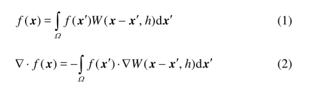
wherexis the position vector,f(x) the field function, ∇⋅f(x) the spatial derivative of field function,W(x-x′,h) the smoothing function, andhthe smoothing length determining the influence area of the smoothing function.

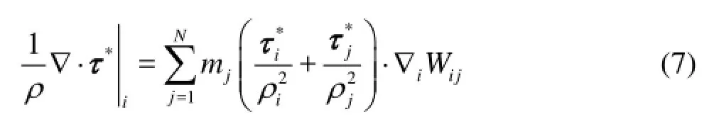
The particle approximation is another key step in the SPH method. In this step, the continuous integral functions will be converted to discretized forms of summations with a finite number of particles that carry individual properties:whereNis the number of particles in the support domain of particlei,ijrthe distance between particleiandj,jρthe density associated with particlej,mjthe mass associated with particlej,Wijthe smoothing function of particleievaluated at particlej, closely related to the smoothing lengthh.
1.2SPH formulations
1.2.1 Navier-Stokes equations in the form of SPH
For dynamic fluid flows, the governing conservation equations can be written as a set of partial differential equations (Navier-Stokes equations). For Newtonian fluids, the viscous shear stress should be proportional to the shear strain rate. The Navier-Stokes equations with laminar viscous stresses are given by

wherevis the velocity vector,pthe pressure, andgthe gravitational acceleration. While in order to handle and capture the turbulence effects, such as eddies and vortex structure in the flow, a Sub-Particle Scale (SPS) turbulence model was developed in Lagrangian particle methods. The SPS approach to modeling turbulence was originally presented by Lo and Shao[9]in their incompressible SPH scheme. Dalrymple and Rogers[10]firstly introduced the SPS model to the weakly compressible SPH scheme. The SPS model added a flat-top spatial filter to the momentum conservation equation.
With a symmetric formulation of Lo and Shao[9], the SPS stresses can be evaluated with
So the SPH form of the SPS momentum conservation equation can be written in SPH notations as follows
The particles are moved based on the velocity

1.2.2 Equation of state
The SPH method introduced the artificial compressibility to use a quasi-incompressible equation of state to model the incompressible flow. The following equation of state for water to model free surface flows presented by Monaghan has been widely used by many applications of SPH[11].
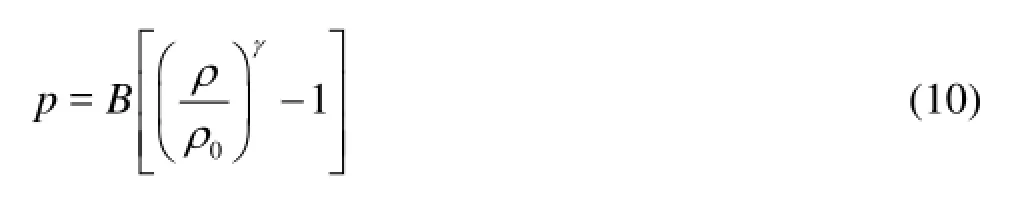
where =γ7 is used in most circumstances,0ρis the reference density and is generally set to the initial density of fluid phase,Bis a problem-dependent parameter, which is also called reference pressure and is given by

cis the artificial sound speed and is commonly chosen based on a scale analysis in order to limit the admissible density variation to 1%. We will clarify the sound speed value used in the following simulations.
2. GPUSPH program
As a meshfree particle method, the SPH could be computationally expensive to compute the massive particle interactions for some large-scale engineering applications. So the acceleration of the SPH using parallel computing technique is really necessary. The powerful parallel nature of GPUs makes them wellsuited tools for advanced scientific modeling. After the CUDA programming language introduced by NVIDIA in the spring of 2007, it becomes really readily accessible for engineers and scientists to use the GPU by extending the C++ language to handle the computing operations of the GPU and its interfacing with the CPU host.
GPUSPH was originally developed by Hérault et al.[12,13], which is programmed in CUDA, C++ and OpenGL based on the SPH methodologies mentioned above. With OpenGL, GPUSPH can display computing results real-time, which is really convenient for identifying local flow features. GPUSPH totally implements all the SPH computing segments (neighbor search, force computation and time integration) on GPU, and has many options for SPH numerical techniques, such as interpolation kernels, density smoo-thing, variable time step, wall boundary treatments, free surface tracking, “XSPH” technique, SPS turbulence mode, etc..
Taking advantage of GPU parallel computing technique, simulations involving millions of particles (or called computational nodes) can be easily achieved using the GPUSPH model, and hence complex local flow features and larger-scale investigation on fluidstructure interactions can be accomplished. Hérault and his co-workers have examined the effectiveness and accuracy of GPUSPH over serial-based SPH computation through benchmarks in Ref.[12,13]. The speedup of force computation part in SPH calculated with GPUSPH using GTX 280 (240 cores) against the performance of a single CPU (Intel Core2 Duo at 2.5 GHz) can be up to 207 times, which is almost proportional to the number of the cores of the GPU video card. So the acceleration of the SPH using the GPU parallel computing technique is promising for largescale engineering applications. Dalrymple and Hérault and their co-workers have successfully used GPUSPH to investigate the water waves in the surf zone on sloping beaches, the breaching of flood walls and the interaction of the flooding waters with obstacles[14,15].
2.1Virtual geometric boundary treatment
Boundary treatment is one of the primary challenges in using the SPH method. For solving this problem, three popular boundary treatments have been presented by the researchers these years[8,11]: (1) fixed solid boundary with repulsive force, (2) ghost-particle boundary, (3) multi-layer virtual particles together with repulsive fixed solid boundary. Among the three boundary treatments, the repulsive boundary is wellsuited to handle the complex geometry wall and can produce a highly repulsive force to prevent the fluid particles from unphysically penetrating through the solid wall. Therefore, we use the fixed boundary treatment for complex buildings and facilities. However, for the outer boundaries of the computational problem domain, instead of establishing the fixed boundaries with particles, we construct the fixed solid wall by using geometric planes[16]. Although this is a more complicated boundary condition to apply, the advantage is that we do not need to initialize fixed boundary particles and the boundaries are mathematical planes. This can be a considerable saving in memory as particle boundaries require a great amount of particles for large-scale problems, especially for GPU computing it could save much video memory.
The plane is defined by a linear equation as follows

The distance of a particle located at (x1,y1,z1) from the plane is calculated by
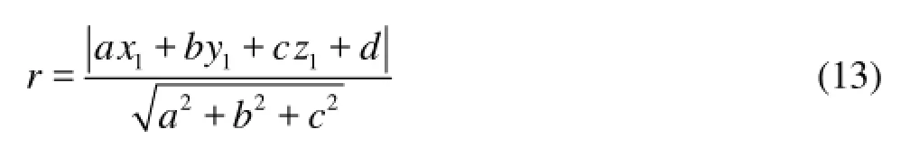
wheredis to determine the distance between the plane and the coordinate axis anda,bandccorrespond to the components of the normal vector of the plane, which is generally set as an unit vector so that the denominator in Eq.(13) is 1. With the distance of a particle located from the plane, we can calculate the repulsive force exerted by the virtual plane according to “Lennard Jones”-like force equation[8,16].
2.2Basic problem objects
In the GPUSPH model, there are a variety of basic objects that can be used to generate problem domain or complex structures. In 2-D cases, the basic objects (in C++ terms, classes) include Point, Vector, Segment, Rect (rectangle) and Circle. In 3-D cases, there are additional objects: Cone, Cube, Cylinder, Sphere and TopoCube. The TopoCube object is used to input the bottom (bathymetry) of the 3-D problem domain via a Digital Elevation Model (DEM) file. Using these basic objects, many types of problem scenarios and complex structures can be constructed.
In this paper, we use the basic Rect object to construct staircases, and use the Cube object, Sphere object, Cylinder object and Cone object together with the Rect object to establish intricate buildings and infrastructural foundations, which will be presented in Section 4.1 and Section 4.2.
2.3Smoothing kernel choice
In the GPUSPH model, there are three kernel functions implemented: quadratic, cubic spline and Wendland quintic. The accuracy of the SPH interpolation generally increases with the order of the polynomial employed in the smoothing function. Gomez-Gesteira et al.[17]discussed the state-of-art smoothing functions and pointed out that the Wendland quintic function can constitute a good choice in terms of computational accuracy and effectiveness, since it provides a higher order of interpolation with a computational cost comparable to the quadratic kernel. Motivated by this, the simulations in this paper use the Wendland quintic smoothing function, which is given by
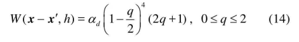
whereαis taken as 7/(4πh2) and 7/(8πh3) in 2-Ddand 3-D spaces, respectively.
2.4Density filter
In the GPUSPH model, two density filters areimplemented: the zeroth-order Shepard filter and the first-order MLS filter[12]. In simulations in this paper we use the MLS approach, which reinitializes the density field using the following equations:

2.5Time stepping scheme
The SPH equations of motion are integrated in time with the predictor-corrector scheme in GPUSPH. This scheme is second order and serves both linear and angular momenta. Take the integration of velocity as an example as follows. The evolution of density and position are similar.
The predictor step predicts the midpoint value
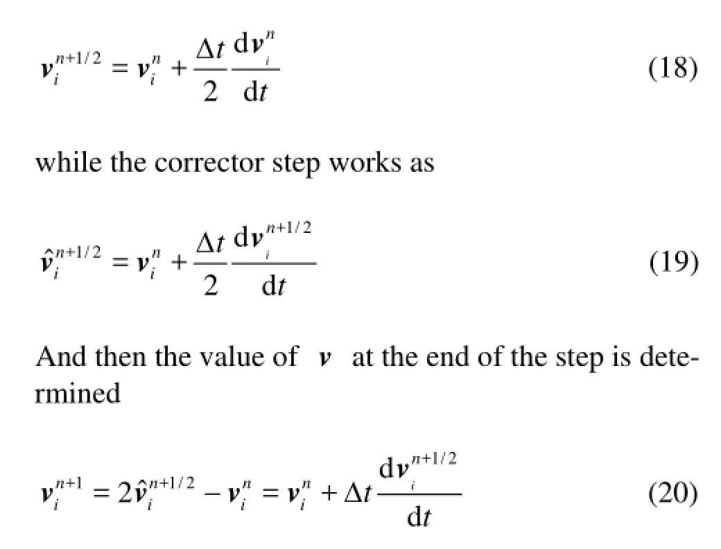
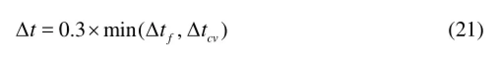
The step size of the time integration is dependent on the forcing terms, the Courant-Fredrich-Levy condition and the viscous diffusion term. Hence a variable time steptΔ is used in the predictor-corrector scheme and is calculated as follows[12]:
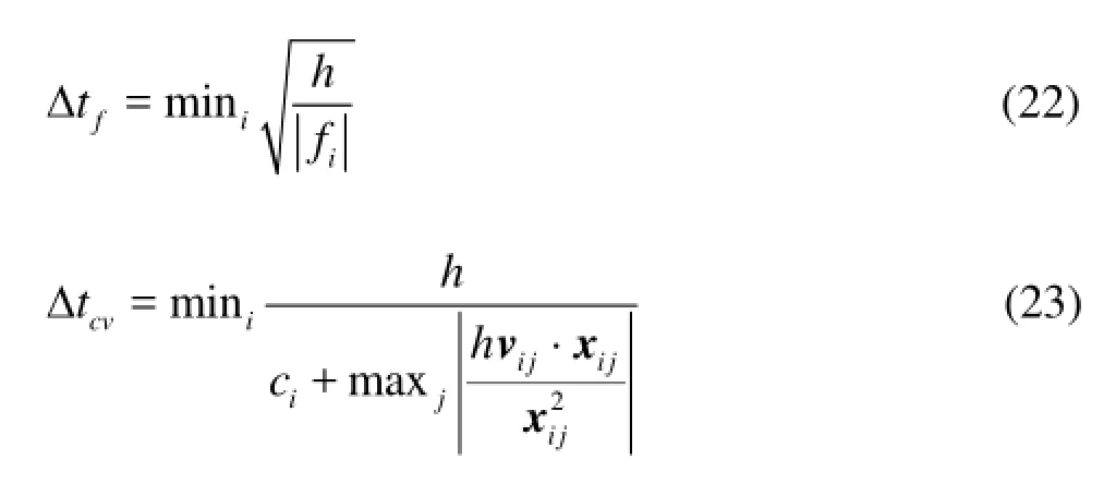
wherevij=vi-vj,xij=xi-xj, andfdenotes the force per unit mass.
3. Validation of dam-break flow through an isolated building
In order to evaluate the accuracy of the SPH modeling of violent dam-break flow, we compare our SPH computed results to a flooding analogue experiment, which was conducted by Soares-Frazão and Zech[18]. This laboratory experiment was to investigate the effects of a single building on dam-break flow propagation.
3.1Experimental set-up
The experiment was carried out in a flume, which is horizontally 35.8 m long and 3.6 m wide with a concrete bed. A 1 m wide rectangular gate is located between two fixed impervious blocks. A 0.8 m×0.4 m rectangular building making an angle of 64owith the channel axis was fixed 3.4 m downstream from the gate. The set-up of the experiment is shown in Fig.1. In initial, the water was set at rest in the 0.4 m depth reservoir behind the gate, and a water layer of 0.02 m depth was set in the downstream bed. Six gages (G1-G6) were used to measure the water levels at different locations with a time step of 0.01 s.

Fig.1 Set-up of the laboratory experiment (m)
3.2The simulations
Our numerical testing platform is a workstaion rack mounting 4×Tesla C2075 cards on as many 2nd generation PCI-Express slots. The system is based on a 2×Intel Xeon X5675 processor with 12 total cores totally (3.06 GHz, 12 MB cache) and 96 GB RAM. Each Tesla C2075 has 480 CUDA cores grouped in 15 multiprocessors, 48KB shared memory per MP, 6.0 GB global memory. The operating system is CentOS 6.3 with CUDA runtime 4.2 installed.
3.3Comparisons of SPH results and experimental data
3.3.1 Global comparisons
We mainly discuss the typical instances of the flow propagation that presents the most complex hydraulic features. From side view and top view, Fig.2 and Fig.3 present the velocity fields at 5.0 s and 10.0 s after the dam break.
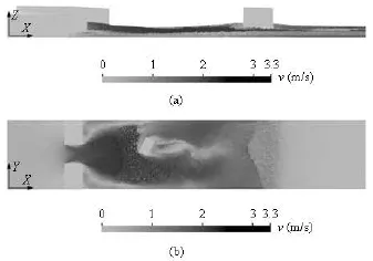
Fig.2 Dam break flood propagation at =t5.0 s
At =t5.0 s, near the isolated building complex flow patterns arise, such as the hydraulic jumps, which are formed by the reflection of the flow against the building and the sidewalls of the channel. From the Fig.2, we observe that the velocities are reduced in the vicinity of the building compared to the upstream of the flow. And also, a wake zone can be identified just behind the building. At =t10.0 s, from Fig.3, we can see that the velocities decrease further, and the wave zone and the hydraulic jumps attenuate slightly. These complex hydraulic features of the results by the SPH model are pretty similar to the measured data by Soares-Frazão and Zech[18]. Moreover, the SPH model can present more 3-D features, such as the vortex at the left down corner of the channel in Fig.2, which can not be tracked by the sparse gages. The vortex of the flow is induced by the reflection of sidewalls of the channel.
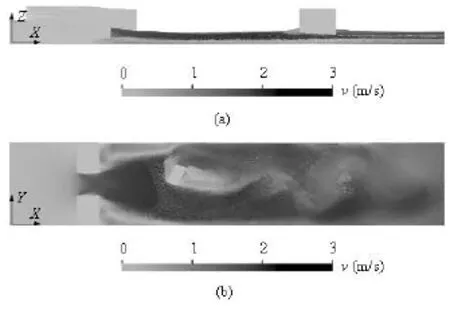
Fig.3 Dam break flood propagation at =t10.0 s

Fig.4 Comparisons of water level evolution at gage G2 between the GPUSPH calculated results with two particle spacings and the experimental data
3.3.2 Comparison of flow levels at selected gages
As was mentioned in Subsection 2.2, we used two particle spacing, P1 and P2 (P1 is 0.01 m and P2 is 0.02 m). We generally assume that the depth of the wet bed of the experimental flume is an integral multiple of the particle spacing. When we use P1 particle spacing, the total particles are up to 12 321 024, which is almost the full load of the four GPU cards. Thus, with our current computer capability we can not try a particle spacing smaller than P1, such as 0.005 m, which is one fourth of the depth of the wet experiment channel.
Figure 4 shows the experimental and computed flow-depths from =t0 s to =t15.0 s at gages G2 (see star sign in Fig.1 for gauge locations). Gage 2 is located upstream from the building and near the right bank of the channel. From Fig.4, we can see that the SPH model both with initial particle spacing P1 and P2 presents the rapid water level rise at the very early times of the wave propagation due to the reflection of the front wave against the right bank of the channel, but the lower resolution initialization produces more oscillations at the later time. That is because the particle spacing of the lower resolution initialization is too big that even two layers of particles are bigger than 0.04 m as the distance between particles can not be compressed too small due to the repulsive force exerted by each other. And also, one layer of particles to initialize the wet bed is so slight that it can result in big fluctuations, see the results at =t9.5 s and =t11 s. With the higher resolution as P1=0.01 m, the results by the SPH model give a very satisfactory agreement with the experimental data during the flow propagation.
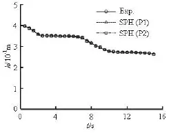
Fig.5 Water level evolution at gage G6 within the reservoir, comparing experimental data to GPUSPH and the SWEs result
Gage 6, located in the reservoir, is used to monitor its emptying and the inflow discharge. From Fig.5, we can observe that the calculated results by the SPH model agrees well with the recorded data in the experiment and the numerical results by Abderrezzak et al.[5], which indicates that the SPH model presents a good inflow discharge through the gate.
Gage 4 is located on the right side of the building and near the right bank of the channel. From Fig.6, we can observe that the SPH model records three reflections of the propagating flow as does the experiment, while quantitatively producing big oscillations after the first hydraulic jump from the timet=2.5 s tot=5 s. These fluctuations are probably induced by the boundary deficiency which exerts excessive repulsive force on the rapid approaching water particles at that period of time. Apart from this period of time, the SPH results agree really well with the experimental data. Moreover, the SPH results are much better than the numerical results calculated by the SWEs model proposed by Abderrezzak et al.[5].It is not surprising that the 3-D SPH model gives much better results than 2-D SWEs models. Indeed, the flow is highly 3-D near the building and especially at the G4 point where the oblique hydraulic jump and the main hydraulic jump merge. This highly unsteady flow makes the assumption of the hydrostatic pressure distribution in the SWEs models invalid.

Fig.6 Water level evolution at gage G4 within the reservoir, comparing experimental data to GPUSPH and SWEs result
Comparisons of the calculated flow depths by the SPH model with the experimental data and numerical results calculated by the SWEs model at selected gages (G2, G4 and G6) show that the SPH model achieves reasonable agreement and reproduces the flow depth oscillations reasonably well. At most of time, acceptable estimates are obtained for the flow level.
4. Dam-break flow through the intricate city layout including underground spaces
The obstacles and underground facilities in the direction of approaching free surface flow may significantly affect the flow evolvement and result in some new flow features. The dam break flood through an isolated building discussed above validates the effects of obstacles. However, the isolated building is simplified to an idealized cube structure. To investigate more complex flow patterns, we establish an intricate city layout including underground spaces. In addition, with different set-ups of the foundations of buildings, we examine the effects of bottom foundation on the dam-break flow propagation.
4.1Set-up of the intricate city layout
With many GPUs coordinated in a GPU cluster, the simulation of large-scale city flooding can be realized, however, at present the GPUSPH is limited by the maximum number of GPUs on a single PCIe bus. Therefore, we examine the small-scale city floodingwith one or couples of GPUs. This small section of a city can illustrate the effects of building layouts and underground spaces on the dam-break flow propagation.

Fig.7 Structure of the complex city layout
The intricate network of city layout consists of several kinds of buildings, underground spaces with stairs, idealized cars and infrastructural constructions (see Fig.7). The city layout is in a channel which is horizontally 15.0 m long and 3.4 m wide. The dam is located at the origin of the channel and the size of the dam is 1.0 m× 3.4 m ×1.0 m. The first row of city layout is 2.0 m away from the dam (in thexaxis direction). The distance between the first two rows of buildings is 0.8 m. The width of the central street is 0.6 m. The height of the buildings in the first row is 2.0 m, and the heights of buildings in the second row are between 2.5 m and 3.0 m. The tallest tower is 5.6 m high. We can set up at most four underground spaces with stairs down to the ground floor in the city layout, and Fig.6 shows the structures of four underground spaces. The first two underground spaces are parallel and is located at (2.8 m, 0.6m, 1.5 m) and (2.8 m, 1.8 m, 1.5 m) respectively. The second two underground spaces are also parallel and located at (4.3 m, 0.6 m, 1.5 m) and (4.3 m, 1.8 m, 1.5 m) respectively. Each underground space has an entrance of 0.3 m× 0.2 m in size and has stairs down to the ground floor. The first stair in each underground space is located at the same horizontal position of the entrance with a size of 0.30 m×0.10 m×0.15 m. Additionally, we make two idealized cars in the central street as white rectangle shows in Fig.7(c).
There are two different foundations of the buildings in the first row of the city layout. One is constructed with staircases, the other is established with four cube cement piles and four cylinder cement piles to elevate parts of buildings above the foundation. In the second row of the city layout, the buildings are in the different shape, i.e., cube buildings and cylinder buildings.
4.2The simulations
4.3Results and discussions
4.3.1 Global flow regimes
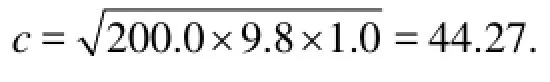
From the top view and side view, Figs.8, 9 and 10 show the propagations of the dam flood in the complex city layout, which are evaluated by the computed velocity fields at =t0.5 s, 1.0 s, 1.5 s after the dam break. The velocity magnitudes in Figs.8, 9 and 10 are the absolute values which are evaluated in linear scale. The different maximum velocity magnitudes in Figs.8, 9 and 10 indicate that the flooding flow
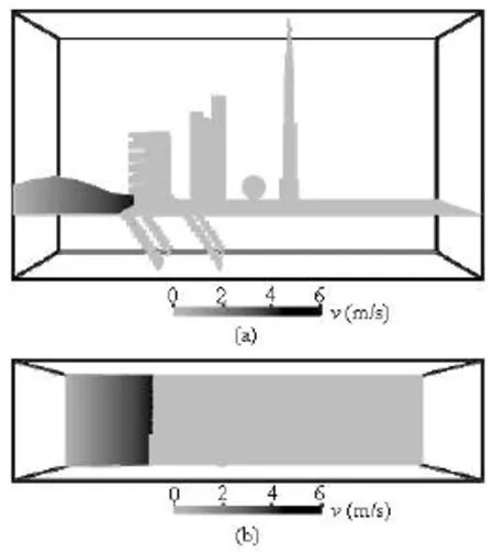
Fig.8 Flood velocity field at =t0.5 s

Fig.9 Flood velocity field at =t1.0 s
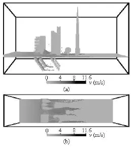
Fig.10 Flood velocity field at =t1.5 s
are getting faster from the dam break starts to the time at =t1.5 s. The pressure evolvement during the flooding propagation is shown in Fig.11 (=t0.5 s, 1.0 s, 1.5 s). To clearly present the variation of pressure field, the pressure value in Fig.10 is evaluated in the logarithmic scale.
Fig.11 Flood pressure field during the flooding propagation
Like the dam break flooding through the isolated building, in the intricate city layout, the upstream hydraulic jumps appear in front of the buildings due to the impact and reflection of the flooding flow against the buildings and sidewalls where the pressure suddenly and locally gets bigger, which is presented in Figs.11(b) and 11(c). And also, wake zones are generated just downstream of every building. More flow patterns arise in the complex city layout due to the different foundations of the buildings and the underground spaces. From Figs.9 and 10, att=1.0 s andt=1.5 s, we can observe that the flooding flow passes through the building with pile foundation moves faster than the buildings built on the staircases, and the flow rises after exiting out from the pile foundation and wave speed increases att=1.0 s (see Fig.9(b)). Because the impact of the flooding flow against the buildings constructed on the staircases is stronger thanthe building built on the pile foundation, it can be observed in Figs.9(b) and 11(b) that more water particles splash out due to the big impact pressure. Hence a bigger hydraulic jump forms in front of the buildings built on the staircases.
Also, we can clearly see that some water flows into the first two underground spaces at =t1.0 s and flows into the other two at =t1.5 s through the stairs. The underground spaces upstream can store more water flow as we observe that more flooding water flows into the two underground spaces under the first row of buildings than the other two under the second row of buildings in Fig.10. From Figs.9, 10 and 11, we know that the velocity of the water flow moving down the staircases is comparatively bigger and the water particles moving down the stairs accentuate big impact on the steps and the bottom of the underground space. Our geometric plane boundary can handle the violent impact well and prevent the water particles from penetrating through the solid walls.
The global propagation regimes of the dam break flow in the intricate city layout fairly well shows the ability of SPH method for 3-D modeling of complex buildings and structures and handling the effects of underground spaces on flooding propagation.
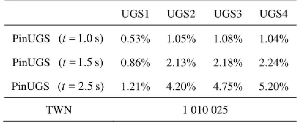
Table 1 Amount of flooding water propagating into one, two, three or four underground spaces
4.3.2 Effects of underground spaces
As was mentioned in Subsection 4.1, we examine four kinds of simulations taking account of one, two, three, or four underground spaces in the city layout. In terms of the scenarios of one, two and three underground spaces, the locations of the underground spaces are as follows: the entrance of the only one underground space is located at (2.8 m, 0.6 m, 1.5 m), the entrances of the two underground spaces are located at (2.8 m, 0.6 m, 1.5 m) and (2.8 m, 1.8 m, 1.5 m) respectively, the entrances of the three underground spaces are located at (2.8 m, 0.6 m, 1.5 m), (2.8 m, 1.8 m, 1.5 m) and (4.3 m, 0.6 m, 1.5 m) respectively. The total number of water particles for each simulation is the same: 1 010 025. Other choices of SPH numerical techniques are the same as the case with four underground spaces. The percentage of the water flow propagating into the underground spaces of each kind of simulation by the time at =t1.0 s, =t1.5 s and =t2.5 s is recorded and given in Table 1.
From Table 1, if we compare the two cases with one underground space and two underground spaces, we can reach a conclusion that basically the amount of flood water which flows into the underground spaces is proportional to the number of the underground spaces if they are in the parallel position along the flow propagation. However, when we compare the three cases with two underground spaces, three and four, we can find it is interesting that the additional one or two underground spaces behind the first row of buildings slightly affects the flow propagation, and stores only 0.55% and 1.0% more water than the city layout with two underground spaces. Therefore, we know that the locations of the underground spaces have significant effect on dam-break flood evolution, and next we verify this conclusion with more simulations based on different set-ups of two underground spaces in the city layout.
The first scenario is to set up two parallel underground spaces in front of the first row of buildings at (2.8 m, 0.6 m, 1.5 m) and (2.8 m, 1.8 m, 1.5 m) respectively. The second scenario sets up two parallel underground spaces just behind the first row of buildings at (4.3 m, 0.6 m, 1.5 m) and (4.3 m, 1.8 m, 1.5 m). The third scenario is that two parallel underground spaces are located behind the second row of buildings at (5.6 m, 0.6 m, 1.5 m) and (5.6 m,1.8 m, 1.5 m) respectively. The last scenario arranges two underground spaces along the central street at (2.8 m, 1.2 m, 1.5 m) and (4.3 m, 1.2 m, 1.5 m) respectively. In a similar manner, we present the percentage of the water flow propagating into the underground spaces by the time at =t1.0 s, =t1.5 s and =t2.5 s in each scenario in Table 2.
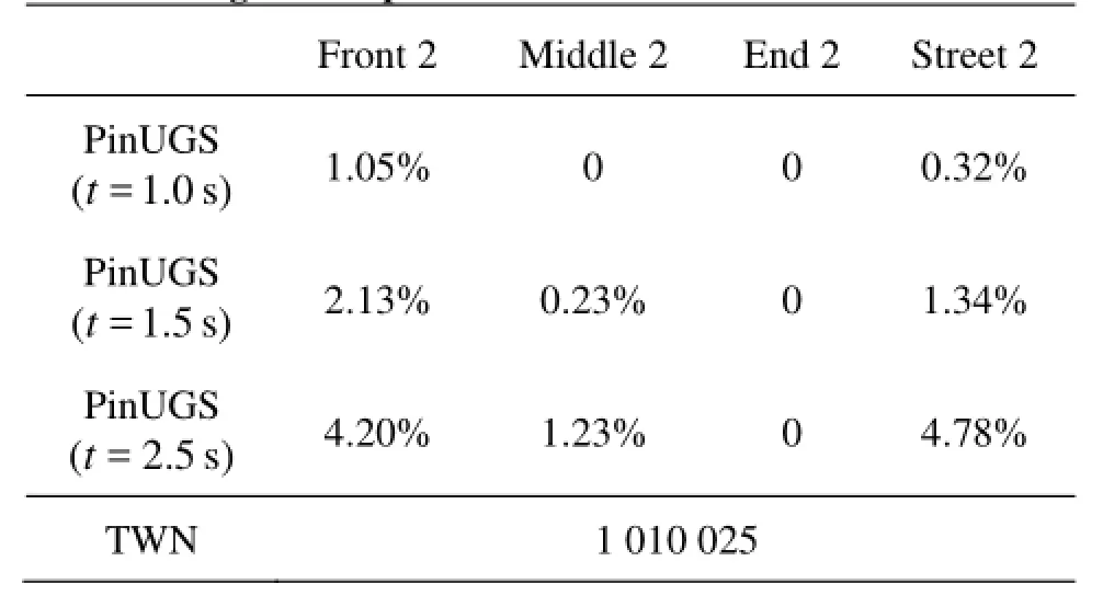
Table 2 Amount of flooding water propagating into two underground spaces with different locations
From Table 2, we can clearly see that the underground spaces located in the open street or upstream of the dam-break flow without the protection by the building layout significantly affect the flood propagation and store much more flooding water. These computed results and findings conform to reality, and ac-cordingly validate our 3-D SPH model.
5. Conclusions
A 3-D model based on the SPH method with GPUs parallel computing, GPUSPH, has been used to investigate the highly unsteady dam break flow through the intricate city layout including underground spaces. Indeed, the present SPH model offers some advantages and presents some findings as follows:
(1) Taking advantage of GPUs parallel computing techniques, simulations involving more than 107particles are achieved.
(2) The present results of GPU-based SPH model qualitatively show the typical 3-D regimes of the dam break flow through the isolated building just like those in the real experiments and reasonably quantitatively agree with experimental data, and are better than the numerical results given by the SWEs model.
(3) We identify the flow features of the flooding water when flowing into underground spaces through stairs, and find that the flooding flow across the building layout with cylinder or cube pile foundation moves faster than across the building layout built on the staircases.
(4) Basically the amount of flooding water which flows into the underground spaces is proportional to the number of the underground spaces if they are parallel along the flood propagation. However, it significantly varies if the underground spaces locate irregularly. The underground spaces located in the open street or upstream of the dam-break flow without the protection by the building layouts significantly affect the flood propagation and store much more flooding water.
Acknowledgement
The author Dalrymple Robert A. was partially supported by ONR, Coastal Geosciences.
[1] TODA K., KURIYAMA K. and OYAGI R. et al. Inundation analysis of complicated underground space[J].Joumal of Hydroscience and Hydraulic Engineering,JSCE,2004, 22(2): 47-58.
[2] TODA K., KAWAIKE N. and YONEYAMA S. et al.
Underground inundation analysis by integrated urban flood model[C].Proceedings of 16th IAHR-APD Congress and 3rd Symposium of IAHR-ISHS.Nanjing, China, 2009, 166-171.
[3] HAN K. Y., KIM G. and LEE C. H. et al. Modeling of flood inundation in urban areas including underground space[C].The 4th International Symposium on Flood Defense.Toronto, Ontario, Canada, 2008.
[4] SOARES-FRAZÃO S., ZECH Y. Dam-break flow through an idealised city[J].Journal of Hydraulic Research,2008, 46(5): 648-658.
[5] ABDERREZZAK K. El K., PAQUIER A. and MIGNOT E. Modelling flash flood propagation in urban areas using a two-dimensional numerical model[J].Natural Hazards,2009, 50(3): 433-460.
[6] SCHUBERT JOCHEN E., SANDERS BRETT F. Building treatments for urban flood inundation models and implications for predictive skill and modeling efficiency[J].Advances in Water Resources,2012, 41: 49-64.
[7] LAI Wencong, Khan Abdul A. Modeling dam-break flood over natural rivers using discontinuous Galerkin method[J].Journal of Hydrodynamics,2012, 24(4): 467-478.
[8] LIU M. B., LIU G. R. smoothed particle hydrodynamics (SPH): An overview and recent developments[J].Archives Computation Methods Engineering,2010, 17(1): 25-76.
[9] LO E. Y. M., SHAO S. Simulation of near-shore solitary wave mechanics by an incompressible SPH method[J].Applied Ocean Research,2002, 24(5): 275-286.
[10] DALRYMPLE R. A., ROGERS B. D. Numerical modeling of water waves with the SPH method[J].Coastal Engineering, 2006, 53(2-3): 141-147.
[11] MONAGHAN J. J. Smoothed particle hydrodynamics and its diverse applications[J].Annual Review of Fluid Mechanics,2012, 44: 323-346.
[12] HÉRAULT A., VICARI A. and DELNEGRO C. et al. Modeling water waves in the surf zone with GPUSPHysies[C].Proceedings of 4th SPHERIC International Workshop.Nantes, France, 2009, 77-84.
[13] HÉRAULT A., BILOTTA G. and DALRYMPLE R. A. SPH on GPU with CUDA[J].Journal of Hydraulic Research,2010, 48(Suppl. 1): 74-79.
[14] DALRYMPLE R. A., HÉRAULT A. and BILOTTA G. et al. GPU-accelerated SPH model for water waves and free surface flows[C].Proceedings of 32nd International Conference Coastal Engineering.Shanghai, China, 2010.
[15] JALALI FARAHANI R., DALRYMPLE R. A. and HÉRAULT A. et al. Turbulent coherent structures under breaking waves[C].Proceedings of 7th SPHERIC Internatinal Workshop.Prato, Italy, 2012, 171-178.
[16] HÉRAULT A., BILOTTA G. and VICARI A. et al. Numerical simulation of lava flow using a GPU SPH model[J].Annals of Geophysics,2011, 54(5): 600-620.
[17] GOMEZ-GESTEIRA M., ROGERS B. D. and DALRYMPLE R. A. et al. State-of-the-art of classical SPH for free-surface flows[J].Journal of Hydraulic Research, 2010, 48(Suppl. 1): 6-27.
[18] SOARES-FRAZÃO S., ZECH Y. Experimental study of dam-break flow against an isolated obstacle[J].Journal of Hydraulic Research,2007, 45(Suppl. 1): 27-36.
10.1016/S1001-6058(13)60429-1
* Project supported by the National Basic Research Development Program of China (973 Program, No. 2012CB719705), the National Natural Science Foundation of China (Grant Nos. 91024032, 70833003).
Biography: WU Jian-song (1985-), Male, Ph. D., Lecturer
猜你喜欢
理科爱好者(教育教学版)(2022年1期)2022-04-14
河北教育(教学版)(2021年10期)2022-01-14
书香两岸(2020年3期)2020-06-29
武大国际法评论(2019年6期)2019-04-09
Defence Technology(2012年3期)2012-07-25

- 水动力学研究与进展 B辑的其它文章
- A three-dimensional hydroelasticity theory for ship structures in acoustic field of shallow sea*
- Experimental study of the interaction between the spark-induced cavitation bubble and the air bubble*
- A preliminary study of the turbulence features of the tidal bore in the Qiantang River, China*
- The calculation of mechanical energy loss for incompressible steady pipe flow of homogeneous fluid*
- Experimental study by PIV of swirling flow induced by trapezoid-winglets*
- Analysis of shear rate effects on drag reduction in turbulent channel flow with superhydrophobic wall*