An Improved Control Vector Iteration Approach for Nonlinear Dynamic Optimization. II. Problems with Path Constraints*

(胡云卿)(刘兴高),**(薛安克)

1State Key Laboratory of Industry Control Technology, Zhejiang University, Hangzhou 310027, China

2Institute of Information and Control, Hangzhou Dianzi University, Hangzhou 310018, China

An Improved Control Vector Iteration Approach for Nonlinear Dynamic Optimization. II. Problems with Path Constraints*

HU Yunqing(胡云卿)1, LIU Xinggao(刘兴高)1,**and XUE Anke(薛安克)2

1State Key Laboratory of Industry Control Technology, Zhejiang University, Hangzhou 310027, China

2Institute of Information and Control, Hangzhou Dianzi University, Hangzhou 310018, China

This paper considers dealing with path constraints in the framework of the improved control vector iteration (CVI) approach. Two available ways for enforcing equality path constraints are presented, which can be directly incorporated into the improved CVI approach. Inequality path constraints are much more difficult to deal with, even for small scale problems, because the time intervals where the inequality path constraints are active are unknown in advance. To overcome the challenge, the l1penalty function and a novel smoothing technique are introduced, leading to a new effective approach. Moreover, on the basis of the relevant theorems, a numerical algorithm is proposed for nonlinear dynamic optimization problems with inequality path constraints. Results obtained from the classic batch reactor operation problem are in agreement with the literature reports, and the computational efficiency is also high.

nonlinear dynamic optimization, control vector iteration, path constraint, penalty function method

1 INTRODUCTION

Owing to the growing popularity of dynamic simulation softwares (e.g., Aspen Dynamics and gPROMS) in chemical engineering processes, operation optimization becomes a problem that needs to be solved urgently. Traditional static optimization methods are no longer suitable for the complex characteristics of modern chemical plants, such as nonlinearity, high dimensionality, and uncertainty. Therefore, more researchers are paying their attentions to using dynamic optimization methods for eliminating bottlenecks and tapping potentials in industrial processes [1, 2].

In the previous paper [3], an improved control vector iteration (CVI) approach was established in detail. The approach can overcome most drawbacks of traditional indirect methods except dealing with path constraints. In this paper, the approach is enhanced further, and both of equality path constraints and inequality path constraints are considered.

Dynamic optimization problems with path constraints are difficult to solve, especially for inequality path constrained problems. The reasons are: the time intervals where one or more active constraints exist are unknown in advance; in a specified time interval, the number of active constraints is also unknown; all the state equations that are described by a set of ordinary differential equations (ODEs) and the active constraints may constitute high-index differential-algebraic equations (DAEs), which are hard to solve currently.

Many researchers have tried to overcome the difficulties [4-10]. In this paper, the l1penalty function and a novel smoothing technique are introduced to enhance the improved CVI approach and make it able to handle path constraints. A significant benefit of using the l1penalty function is that the solution of the original dynamic optimization problem can be approximately obtained by solving a sequence of unconstrained nonlinear programming problems (NLPs). However, the l1penalty function is not differentiable (i.e., non-smooth), so that many sophisticated NLP algorithms such as BFGS can not be used directly. To remedy the deficiency, a new-emerging smoothing technique given by Meng et al. [11] is applied, and the relationship between the original problem and the smoothed penalty problem is also elaborated, resulting in a concomitant numerical algorithm for nonlinear dynamic optimization problems with path constraints.

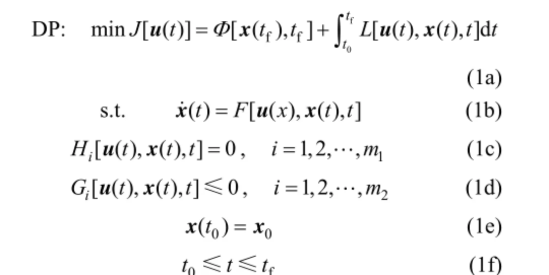
2 PROBLEM FORMULATION

The nonlinear dynamic optimization problems with path constraints can be formulated mathematically as follow:

3 APPROACH DESCRIPTION

3.1 Dealing with equality path constraints

Equality path constraints are relatively much easier to deal with than inequality path constraints. Two effective ways can be incorporated into the improved CVI approach directly. The first one is suggested by Vassiliadis [5] that all the equality path constraints are enforced by minimizing the integral of their squared residual, thus DP becomes:

When J[u(t)] reaches its minimum, the last term in Eq. (2a) should be zero, consequently the equality path constraints Eq. (1c) are satisfied. The second one is to treat Eq. (1b) and Eq. (1c) as a differential-algebraic equations (DAEs) system (the index of the DAEs system should be less than 3), which can be solved by state-of-art DAE solvers [12].

3.2 Penalty function method for dealing with inequality path constraints

Inequality path constraints are very difficult to handle, even for small-scale problems [10]. The idea of penalty was mentioned early in Bryson and Ho [13], where the inequality path constraints were suggested being enforced by augmenting the original objective function as

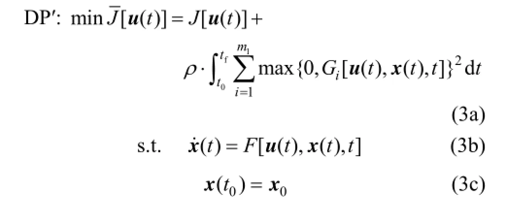
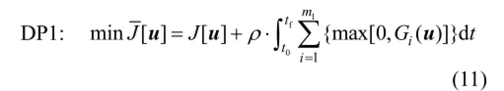
where ρ is the penalty parameter. In fact, this form applies the quadratic penalty function which is not exact, that means ρ should be very large when the solution of DP′ can be taken as an approximate solution of DP. To remedy this flaw, the l1exact penalty function is used, resulting in the new problem DP1:

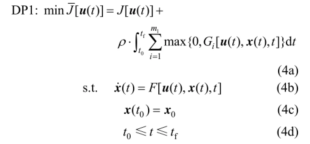
For the exactness of the l1penalty function method, there exist a threshold value ρ∗for the penalty parameter ρ, that for all ρ ρ∗> , the solution of DP1 is exactly the solution of DP [14]. This favorable property can avoid the possible numerical difficulties caused by the very large value of ρ in DP′.

3.3 Smoothing technique

Although the l1penalty function is exact, it is not differentiable, which means the sophisticated gradient based NLP algorithms can not be used to solve DP1. In this study, a novel smoothing technique [11] is adopted to overcome this drawback.

The non-differentiable operator max{0, y} can be equivalently expressed by Eq. (5a):

Recently, Meng et al. [11] proposed a smooth function that can approximate p(y) with artificially precision:

where the parameter a should be greater than 1. For the constrained NLP problem in Eq. (6), the l1penalty function is expressed in Eq. (7) and the smoothed l1penalty function is expressed in Eq. (8).

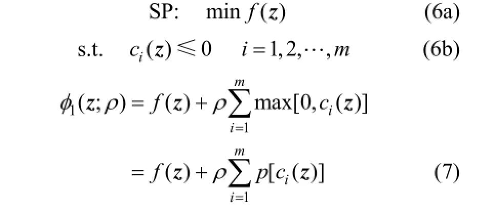
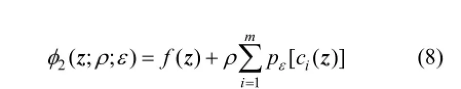
Accordingly, two penalty problems in Eqs. (9) and (10) are obtained, both of them are unconstrained NLP problems:

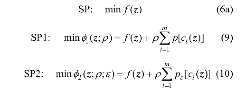
Meng et al. [11] also proved the following theorems, where ε is called the smoothing parameter.

Definition 1 A vector zεis ε-feasible to SP if

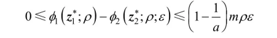
Theorems 1 and 2 indicate that when ε is sufficiently small, the solution of SP2 is an approximate solution of SP1.

3.4 Solve the problem DP with the smoothed penalty method

Suppose u(t) has been discretized in the time horizon, and the state variables x(t) have been calculated by solving Eq. (1b) and Eq. (1e) with a set of given control variables (this is reasonable in the iterative solution process, please see the implementation structure in the first paper [3]), then DP1 becomes:

Applying the novel smoothing technique to DP1, DP2 is produced:

It is surprising to find that the relationship between the problems DP, DP1 and DP2 is the same as the relationship between SP, SP1 and SP2. In other words, for all ρ> ρ∗, the solution of DP2 is an approximate solution of DP.

3.5 Algorithm outline

The improved CVI approach is enhanced by applying the smoothed l1penalty function, its structure is sketched in Fig. 1, and the corresponding numerical algorithm is given below:

Step 1 Set initial penalty parameter ρ and initial smoothing parameter ε.

Step 2 Set tolerances ε1for Adams algorithm, ε2for BFGS algorithm, ε3for feasibility, choose the time interval number N.

Step 3 Assign the initial guess for control variablesaccording to experience or priori knowledge about the problem. Set the number of iteration k=0.

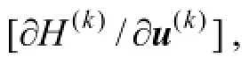
Step 4 Integrate the state and adjoint equations by Adams algorithm, thusJ[u(k)] andare obtained. Go to Step 5.

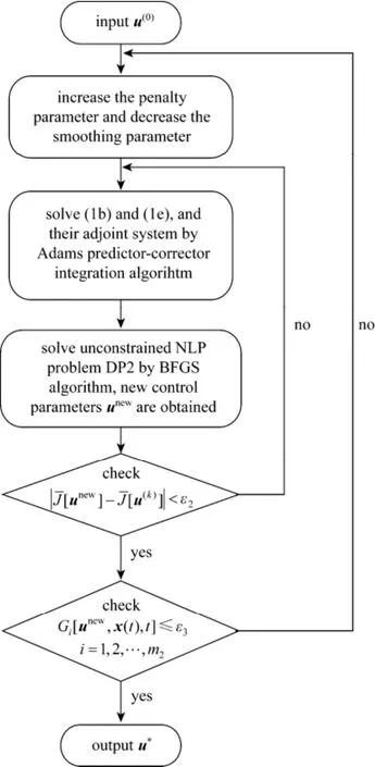
Figure 1 The structure of the improved CVI approach

4 CASE TESING

The batch reactor operation problem with the parallel reaction mechanism: A→B, A→C (the objective is to find the optimal temperature operating policy below 412 K that maximizes the yield of B), is tested again with additional path constraints (for more background about the problem please refer to [3]). The computing platform consists of Pentium E6550/2.93GHz CPU and DDRII/1000MHz system memory. The desired integration tolerance ε1and the optimization tolerance ε2are set to 10−6, ε3is set to 10−4. The parameter a in Eq. (5b) is set to 2.

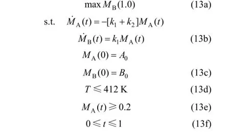
Bloss and Biegler [7] added a state inequality path constraint on this problem, that the yield of A should never be less than 0.2, the modified problem is formulated as The initialconditionsare:A0=1,=0,ρ=1, ε=5×c=10, d=0.5, and=2 uniformly. The algorithm in Section 3.5 is used to solve this problem and Table 1 summarizes the results. It can be s e en there are 3 times of penalty in the solution proce s s. For instance,when ρ=1 and ε=5×the o b je ctivefunction value is 0.5631 while the error is gr e a ter thanthenthe penalty parameter and the smoothing parameter are updated by the rules: ρ= 10⋅ρ and ε=0.5⋅ε, respectively, and the algor i t h m res t a rts fromStep4. When ρ=100 and ε= 1 . 2 5 ×t h e algorithmstops with theobjective function value of 0.5347. The solution process needs 37 BFGS iterations in all and 7.25 s.

Figure 2 shows the change of control profile in the solution process, and Fig. 3 shows the optimalstate variables. In Fig. 2, the upper bounds for k1and k2are the same as in the first paper [3], meaning that the path constraint Eq. (13d) is satisfied. From Fig. 3 it can be seen that, the yield of A only equals to 0.2 at tf, implying the path constraint Eq. (13e) is satisfied well during the whole operation process. Furthermore, the optimal objective function value of 0.5347 is close to the result by Bloss and Biegler [7], which demonstrates the effectiveness of the proposed algorithm.

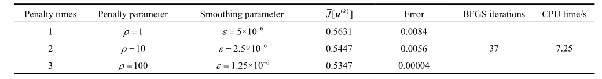
Table 1 Results for the constrained batch reactor problem

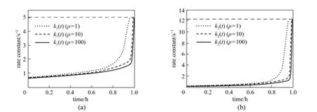
Figure 2 Control profile in the solution process

Figure 3 Optimal state profiles

5 CONCLUSIONS

This paper aims to handle path constraints in the framework of the improved CVI approach. Equality path constraints can be enforced by minimizing the integral of their squared residual, or taken with the differential equations together as a DAEs system. Inequality path constraints are incorporated into the original objective function and enforced gradually by penalty function method. In order to use the sophisticated NLP algorithms such as BFGS, a novel smoothing technique is used to make the l1penalty function differentiable. Based on the relationship between the original problem and the smoothed problem, an efficient numerical algorithm for path constrained dynamic optimization problems is elaborated. The changes of the control profiles in the solution process are also illustrated. In addition, the low computational cost indicates the algorithm may have more potential in practical implementations.

REFERENCES

1 Biegler, L.T., Nonlinear Programming: Concepts, Algorithms, and Applications to Chemical Processes, SIAM, Philadelphia (2010).

2 Woranee, P., Paisan, K., Amornchal, A., “Batch-to-batch optimization of batch crystallization processes”, Chin. J. Chem. Eng., 16 (1), 26-29 (2008).

3 Hu, Y.Q., Liu, X.G., Xue, A.K., “An improved control vector iteration approach for nonlinear dynamic optimization. I. problems without path constraints”, Chin. J. Chem. Eng., 20 (6), 1053-1058 (2012).

4 Jacobson, D.H., Lele, M.M., “A transformation technique for optimal control problems with a state variable inequality constraint”, IEEE Trans. Auto. Control, 14 (5), 457-464 (1969).

5 Vassiliadis, V.S., “Computational solution of dynamic optimization problems with general differential-algebraic constraints”, Ph.D. Thesis, University of London, London, UK (1993).

6 Feehery, W.F., “Dynamic optimization with path constraints”, Ph.D. Thesis, MIT, Boston, USA (1998).

7 Bloss, K.F., Biegler, L.T., Schiesser, W.E., “Dynamic process optimization through adjoint formulations and constraint aggregation”, Ind. Eng. Chem. Res., 38 (2), 421-432 (1999).

8 Bell, M.L., Sargent, R.W.H., “Optimal control of inequality constrained DAE systems”, Comput. Chem. Eng., 24 (11), 2385-2404 (2000).

9 Chen, T.W.C., Vassiliadis, V.S., “Inequality path constraints in optimal control: a finite iteration ε-convergent scheme based on pointwise discretization”, J. Process. Contr., 15 (3), 353-362 (2005).

10 Luus, R., “Handling inequality constraints in optimal control by problem reformulation”, Ind. Eng. Chem. Res., 48 (21), 9622-9630 (2009).

11 Meng, Z., Dang, C., Jiang, M., Shen, R., “A smoothing objective penalty function algorithm for inequality constrained optimization problems”, Numer. Func. Anal. Opt., 32 (7), 806-820 (2011).

12 Hindmarsh, A.C., Brown, P.N., Grant, K.E., Lee, S.L., Serban, R., Shumaker, D.E., Woodward, C.S., “SUNDIALS: Suite of nonlinear and differential/algebraic equation solvers”, ACM Trans. Math. Software, 31 (3), 363-396 (2005).

13 Bryson, A.E., Ho, Y.C., Applied Optimal Control: Optimization, Estimation, and Control, Taylor & Francis, New York (1975).

14 Han, S.P., Mangasarian, O.L., “Exact penalty functions in nonlinear programming”, Math. Program., 17 (1), 251-269 (1979).

Received 2012-08-04, accepted 2012-10-08.

* Supported by the National Natural Science Foundation of China (U1162130), the National High Technology Research and Development Program of China (2006AA05Z226), and Outstanding Youth Science Foundation of Zhejiang Province (R4100133).

** To whom correspondence should be addressed. E-mail: liuxg@iipc.zju.edu.cn