An Adaptive Discretization of Incompressible Flow using Node-Based Local Meshes

Weiwei Zhang,Yufeng Nie,Li Caiand Nan Qi

1 Introduction

Unstructured mesh adaptation is now widely used in numerical simulations to improve the accuracy of solutions as well as to capture the behavior of physical phenomena.Specifically,for the Stokes problem,the adaptive analysis has two procedures:a posteriori error estimation and mesh adaptivity based on the result of error estimation.In the last few decades,how to derive a posteriori error estimates for the Stokes equations has received much attention,and many researchers have acquired quantities of good results,see Refs.[Babuvška and Rheinboldt(1978);Verfürth(1989,1991);Kay and Silvester(1999);Ervin and Phillips(2006);Liao and Silvester(2012)]and references therein.

The performance of adaptive methods for PDEs depends not only on the error estimators,but also on techniques used for constructing adaptive meshes.Successful implementation of the adaptive strategy can improve the accuracy of numerical approximations and decrease the computational cost.In the past two decades,a large number of research works relevant to the adaptive mesh generation in different research and application fields occurred,see for instance[Ju,Gunzburger,and Zhao(2006);Huang,Qin,Wang,and Du(2011);Biboulet,Gravouil,Dureisseix,Lubrecht,and Combescure(2013)]for elliptic problems and[Picasso(2003)]for parabolic problems.In addition,the authors of Refs.[Boussetta,Coupez,and Fourment(2006);Labergère,Rassineux,and Saanouni(2011)]have proposed an adaptive meshing frame for forging simulation which is based on an iterative mesh improvement by local changes.Although adaptive mesh refinement techniques are availablefortheStokesequations[Zheng,Hou,andShi(2010);He,Xie,andZheng(2010);Araya,Barrenechea,and Poza(2008)],the mesh adaptation algorithms for the Stokes problems has not been widely studied.In Refs.[Zheng,Hou,and Shi(2010);He,Xie,and Zheng(2010)],the finite element software FreeFem++[Hecht(2012)]is applied by using the mesh generatorbamg[Hecht(1998)]to create successivelyre finedmeshes.Basedonthebisectiontechnique,thebamgcansubdivide some selected elements to obtain a new mesh quickly.However,it needs to take appropriate measures to remove hanging nodes,coordinating the new mesh.Besides,the smoothness procedure is necessary for thebamgbetween the refined and nonrefined areas.In addition,a sequence of refined meshes are provided by using the mesh generatorTriangle[Shewchuk(2005)]for the generalized Stokes problems[Araya,Barrenechea,and Poza(2008)].In general,the mesh adaptation methods can be classified into three categories:

The performance of adaptive methods for PDEs depends not only on the error estimators,but also on techniques used for constructing adaptive meshes.Successful implementation of the adaptive strategy can improve the accuracy of numerical approximations and decrease the computational cost.In the past two decades,a large number of research works relevant to the adaptive mesh generation in different research and application fields occurred,see for instance[Ju,Gunzburger,and Zhao(2006);Huang,Qin,Wang,and Du(2011);Biboulet,Gravouil,Dureisseix,Lubrecht,and Combescure(2013)]for elliptic problems and[Picasso(2003)]for parabolic problems.In addition,the authors of Refs.[Boussetta,Coupez,and Fourment(2006);Labergère,Rassineux,and Saanouni(2011)]have proposed an adaptive meshing frame for forging simulation which is based on an iterative mesh improvement by local changes.Although adaptive mesh refinement techniques are [Zheng,Hou,and Shi(2010);He,Xie,and Zheng(2010);Araya,Barrenechea,and Poza(2008)],the mesh adaptation algorithms for the Stokes problems has not been widely studied.In Refs.[Zheng,Hou,and Shi(2010);He,Xie,and Zheng(2010)],the finite element software Free Fem++[Hecht(2012)]is applied by using the mesh generatorbamg[Hecht(1998)]to create successivelyrefined meshes. Based on the bisection technique,thebamgcansubdivide some selected elements to obtain a new mesh quickly.However,it needs to take appropriate measures to remove hanging nodes,coordinating the new mesh.Besides,the smoothness procedure is necessary for thebamgbetween the refined and nonrefined areas.In addition,a sequence of re fined meshes are provided by using the mesh generatorTriangle[Shewchuk(2005)]for the generalized Stokes problems[Araya,Barrenechea,and Poza(2008)].In general,the mesh adaptation methods can be classified into three categories:

(i)p-refinement in which the same elements are used but the order of interpolation is increased.

(ii)r-refinement in which the connectivity of the mesh remains unchanged but the nodes are moved to increase mesh density in certain locations.

(iii)h-refinement in which the element sizes are varied.It can be further divided into two categories:

·Mesh subdivision where individual elements are subdivided without changing their original position.

·Complete regeneration by adaptive remeshing.

For the above three procedures, Nithiarasu et al. [Nithiarasu and Zienkiewicz(2000)] point out that for the method (i), as most fluid mechanics problems involvean explicit time marching algorithm, higher order element is not popular. Sincenew nodes are not added in the method (ii), the accuracy of the solution derivedby this method is limited by the initial number of nodes and elements. As to themethod (iii), both mesh subdivision and adaptive remeshing are suitable for most ofthe fluid mechanics problems. While in the mesh subdivision method, it is difficultto take into account simultaneously the bisection and the need of anisotropy of themesh when generating anisotropic mesh, and further difficulty arises in the couplingof refined and original elements [Nicolas and Fouquet (2013)]. However, theabove difficulties can be avoided by using the adaptive remeshing method, in whichthe whole domain is remeshed based on the a posteriori error estimation computedfrom the previous solution.

Motivated by the works[Chen,Nie,Zhang,and Wang(2012);Nie,Zhang,Qi,and Li(2014)],in this paper we present the first effort in designing an adaptive node-based local mesh refinement method-BLMG to solve the Stokes problems based on the error estimation.In previous work,the node placement method[Liu,Nie,Zhang,and Wang(2010);Zhang,Nie,and Li(2012);Nie,Zhang,Qi,and Li(2014)]and its acceleration strategies[Qi,Nie,and Zhang(2014)]have been studied,where the node size function is usually given as input information.This is inadvisable to predefine the size functions to generate variable density meshes for the solution of flow problems with local singularities.In this study,through adopting suitable a posteriori error estimator and mesh size modification technique,together with the node-based local mesh generation strategy,the BLMG method can be used to deal with the Stokes problem with the low-order mixed FEM[Bochev,Dohrmann,and Gunzburger(2006);Li and He(2008);He,Xie,and Zheng(2010);Zheng,Hou,and Shi(2010)].

It’s well known that the lowest equal-order finite element pairs do not satisfy the inf-sup condition which guarantees the convergence of the FE-discretization[Cuvelier,Segal,and Van Steenhoven(1986)].Here a stabilized approach[Bochev,Dohrmann,and Gunzburger(2006)]to the Stokes equations is used by adding a stabilized termG(p,q)to the variational formulation.The obtained discretization form can satisfy the inf-sup condition and thus has a unique solution.Next,a brief outline of the BLMG-based adaptive stabilized method is given.Initially,a coarse Delaunay triangular mesh with a uniform size is constructed.Then,the iterative loops of finite element solution,error estimate,modification of mesh size function and mesh refinement are executed. At each refinement level, a new mesh size fieldis firstly defined based on the obtained error estimation. Then according to Newton’ssecond law of motion, the nodes are moved into a near-optimal configurationwith dynamic simulation. Finally, the patch of elements around each node is builtvia the BLMG method, and the union of the patches is a Delaunay triangulation.The combination of adaptive BLMG with the low-order mixed FEM is particularlyefficient and combines some best algorithmic features of each. In addition, the aposteriori error indicator reported in Ref. [He, Xie, and Zheng (2010)] is used andverified to be equivalent to the discretization error.

The paper is organized as follows.In Section 2,the adaptive BLMG method is described in detail,consisting of how to modify the mesh size based on a posteriori error estimation,how to optimize nodal distribution,and how to generate the nodebased local meshes.In Section 3,the adaptive mesh method is applied to the Stokes problems,some well-known results of the stabilized mixed low-order FEMs,and the error estimates used in this study are introduced.In Section 4,numerical experiments are carried out to verify the good stability and accuracy of our method.Finally,some conclusions are obtained in Section 5.

2 Adaptive mesh strategy

For any adaptive finite element method,there are two key points,namely the error estimator of the computed finite element solution and the mesh adaptive strategy to adjust the mesh based on the estimated errors.In this study,two types of error estimators are used which will be briefly described in Section 3.1.As for the mesh adaptation strategy,we mainly focus on the node-based local mesh generation method BLMG at each refinement level.

Step 1:Develop a new mesh sizeh(l+1)according to a posteriori error estimators and the current mesh sizeh(l);

Step 2:Generate the new mesh verticesusing the node placement method by bubble simulation;

2.1 Relationship between a posteriori error estimator and mesh size

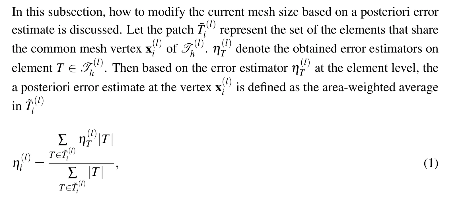
where|T|denote the area of elementT.After obtaining the error estimate at each mesh vertex,the new size function can be uniquely determined by a piecewise linear functionh(l+1)on Ω,such that for any vertex

Algorithm 1 Node placement by bubble simulation Require:The desired mesh size function h(x,y),(x,y)is the position coordinate of nodes.Require:The current mesh vertices{xi}Ni=1.1:Establish an adjacency list for each bubble which stores the information of its neighboring bubbles.2:Solve the motion equations of the bubbles iteratively using the Euler’s predictor-corrector numerical method.3:Update the adjacency lists every k iterative steps(k=5).4:Adjust the number of the bubbles based on the overlap ratios per a fixed iterative step.5:Check if the termination condition is satisfied.If so,terminate;otherwise,go back to step 2.

2.2 Node placement by bubble simulation

After determining the new size function,the current nodes will be optimized by bubble simulation[Nie,Zhang,Liu,and Wang(2010);Qi,Nie,and Zhang(2014)]via inserting or deleting nodes iteratively,such that the refined or coarsened nodes satisfy the requirement of the new size function.The process of the node placement is shown in Algorithm 1,and a brief description is given in the following.

At the beginning of the simulation,the current mesh verticesered as the centers of the bubbles,and the radius of the bubble centered atHere each bubble is dragged by two types of forces,i.e.,the interaction force from neighboring bubbles and the viscous damping force from the system.

The interaction force for two neighboring bubbles,much like the van der Waals force,is approximated by[Shimada and Gossard(1998)]

which tries to maintain the ideal distance between two bubbles by exerting a repelling force when they are too close,or an attracting force when they are not too distant,if two bubbles are far enough,there will be no interaction between them.Herewis the ratio of the real distance and the desired distance between two bubbles,and the desired distance for two bubblesiandjis defined aswhich is the sum of the radii of the two bubbles.

Meanwhile,the damping force from the system is denoted by−,which makes the bubble system converge to a stable con figuration,wherec˜ is the damping coefficient.According to Newton’s second law of motion,the motion equation of each bubble is

wherefijis the interaction force from the neighboring bubblej.The information of neighboring bubbles is stored in an adjacency list related to bubblei,andn(l)denote the size of the adjacency list.About the establishment and update of the adjacency list associated with each bubble,we can refer to[Nie,Zhang,Liu,and Wang(2010)]for details.

To solve the second-order differential equation system(5),adopting high-precision numerical methods (such as fourth-order Runge-Kutta method) will result in a highquality node set.However,this will inevitably lead to large time consumption due to the dynamic simulation.Thus,it is necessary to choose a lower complexity numerical method which also ensures the quality of node sets simultaneously.Instead of the fourth-order Runge-Kutta method,a second-order Euler’s predictor-corrector method is used here to obtain the position coordinates of bubbles at the next step.

During dynamic simulation,the overlap ratio[Shimada and Gossard(1998);Nie,Zhang,Liu,and Wang(2010)]is defined for each bubble to control the number of bubbles,

whereriandrjdenote the ideal radii of bubblesiandj,respectively,i.e.,andis the real distance between the centers of bubblesiandj.In fact,the overlap ratio indicates the number of neighboring bubbles of each bubble.Hence,through setting threshold values of the overlap ratio for the bubbles on a line,on a surface or in an internal volume,we compute the overlap ratio per a fixed iterative step.The bubbles with large overlap ratios will be deleted,while the ones with small overlap ratios will have new bubbles added in its neighborhood.In this manner,the population of bubbles can be controlled dynamically.

The termination condition in previous study[Nie,Zhang,Liu,and Wang(2010)]is usually set to be that the iterative process reaches a prescribed round number,which is usually an empirical value.In this study,the termination condition is logically set such thatN1−N2≤0.5%×N1is satisfied for twice,whereN1andN2are the number of nodes before and after this round of simulation,respectively.By adopting the less complexity numerical method and the improved termination condition mentioned above,the computing cost decrease significantly by 50%,meanwhile,the average quality of the corresponding triangulation is maintained 90%substantially[Qi,Nie,and Zhang(2014)].

2.3 Bubble-type local mesh generation method

Based on the node set generated by the bubble simulation,how to connect these nodes to construct a triangulation of the analysis domain is discussed in this subsection.Firstly,some notations are introduced in the following.In a Delaunay triangulation,the elements which share one common nodePcompose an element patch denoted by,and the common nodePis viewed as acentral node.Each element in the patchis called asatellite elementof the central nodeP,and a node of a satellite element,other than the central node is referred to as asatellite node,which is illustrated in Fig.1.For each central node,the corresponding element patch can be generated by the BLMG method described in the following.

The node placement method mentioned above provides not only a high-quality node set,but also the adjacency list of each node which stores the information of the neighboring nodes.Meanwhile,the adjacency list related to each node includes[Chen,Nie,Zhang,and Wang(2012)]:

Figure 1:Element patchassociated to a central node P.

·all of the satellite nodes in the corresponding Delaunay triangulation;

·a small number of non-satellite nodes(no more than 2).

In fact,in a Delaunay triangulation,mesh edges are built by connecting the central nodes and their satellite nodes.Since both the satellite and non-satellite nodes lie in the adjacency list,the question is how to delete the non-satellite nodes in the adjacency list of each node.In the following,a simple strategy of removing the non-satellite nodes is given as follows:

(i)Connect every central node with all its adjacent nodes from its corresponding adjacency list.

(ii)Sort the nodes from the adjacency list in a counterclockwise order.Taking the central nodePas an example,we can get the sequence like ···Pj−1,Pj,Pj+1···which is shown in Fig.2.

(iii)Check each node in the sequence whether a satellite node of the central nodePin turns.When checking the nodePjwhether a satellite node ofP,we firstly need to judge whether or not the nodesPj−1andPj+1lie in each other’s adjacency lists.If not,the nodePjis a satellite node of the central nodeP.Otherwise,according to step(i),the nodesPj−1andPj+1are connected into the edgewhich intersects with the edgethen Delaunay criteria can be used to check the position relationship between the nodePjand the circumscribed circle of ∆PPj−1Pj+1.IfPjlies outside the circumscribed circle of∆PPj−1Pj+1,thenPjis a non-satellite node of the central nodeP,deletingPjfrom the adjacency list;otherwise,Pjis a satellite node ofP.

After deleting the non-satellite nodes of each central node,the adjacency list corresponding to one central node only consists of all its satellite nodes.Then the set of the satellite elements associated with each central node is built which can be seen in Fig.1.Local meshes around each node are generated under the constraints that the edges of satellite elements do not cross each other.If this condition is not satisfied,the satellite elements are referred to as inconsistent,as shown in Fig.3.However,the inconsistency phenomenon which probably occurring in the BLMG process is circumvented in virtue of the uniqueness of the Delaunay partition which has been verified in Ref.[Nie and Chang(2006)].This ensures that the union of the satellite elements is a Delaunay triangulation of the domain.

The most significant difference between the BLMG and the local mesh generationtechniques in Ref. [Fujisawa, Inaba, and Yagawa (2003)] is that the latter beginsby appropriately distributing the nodes in the computational domain, i.e., nodalcoordinates and nodal density information are given as input information. However,how to generate suitable nodes in Ref. [Fujisawa, Inaba, and Yagawa (2003)] is notmentioned. Moreover, the authors of Ref. [Fujisawa, Inaba, and Yagawa (2003)]take much effort to search satellite nodes for local mesh generation, nevertheless,the searching process is completely avoidable in the BLMG method because theadjacency list of each node contains the total information of the neighboring nodes.

T.Coupez et al.[Boussetta,Coupez,and Fourment(2006)]also adopt local mesh refinement technique which is considered as the improvement of an existing mesh rather than a complete rebuilding process.In Ref.[Boussetta,Coupez,and Fourment(2006)],some elements are iteratively selected and removed by using appropriate local criteria,and local refinement is implemented in the current visited subdomain.This indicates that the selection of remeshing areas is partially affected by manual intervention,and a special treatment may be needed for the transition between two different levels of refinement.Also,the transition region must be carefully set to avoid the sharp jump of mesh size or occurring excessive refinement.Compared to T.Coupez’s approach,the BLMG-based adaptive method uses a strategy based on particles to move mesh points and reconstruct a new triangulation.There fining/coarsening of mesh is completely determined by the size function based on a posteriori error estimation.Meanwhile,this technique works identical for 1D,2D and 3D problems.For any dimension,the rules for moves of particles and the node connection scheme are the same,and 3D BLMG-based adaptive method is a future research topic.

3 Application to Stokes problems

In this study,the BLMG-based adaptive method is applied to solve the homogeneous Dirichlet boundary value problem for the Stokes equations

where Ω represent a polyhedral domain inR2with a Lipschitz continuous boundary∂Ω,u is the velocity vector,pis the pressure,and f is the prescribed body force.The standard variational formulation of(8)is given by: find(u,p)∈(V,S)satisfying

with the inner product(·,·)inL2(Ω).The norm and seminorm inHk(Ω)are denoted by||·||kand|·|k,respectively.

Let P0,P1denote the constant polynomials space and the linear polynomials space,we put

The lowest equal orderC0velocity and pressure pair is

As we know,the above finite element pair does not satisfy the discrete inf-sup condition.

Now,the stabilized low-order mixed finite element method for Stokes equations in[Bochev,Dohrmann,and Gunzburger(2006)]is: find(u,p)∈(V,S)such that

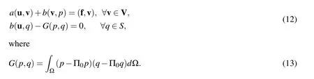
Here Π0:L2R0is the orthogonal projection operator.By restricting(12)to the finite element spaces we can obtain the stabilization method.That is: find(uh,ph)∈(Vh,Sh)such that

It has been proved in Ref.[Bochev,Dohrmann,and Gunzburger(2006)]that(14)is a stable variational problem.

3.1 Error estimator

Two residual a posteriori error estimators at the element level are defined,see[He,Xie,and Zheng(2010)].For simplicity,leteh=u−uhand εh=p−ph,where(u,p)is the solution of the Stokes equations(8),and(uh,ph)is the solution of the stabilized mixed problem(14).In the residual error estimators,one is related to the stabilization term,the other is based on the residue of the finite element discretization.

(i)The first kind of indicator

(ii)The second kind of indicator

where I is the identity operator,P0denote theL2-projection ontoP1,and the[·]Jdenote the jump in the normal flux across the edgee.Then the total a posteriori error is

In order to illustrate that the mesh refinement strategy presented in this study is independent of the choice of the specific error estimator,the projection error estimator ηPis also used in comparison with the residual error estimator ηR,where ηP

Note that the projection operator Π1:L2(Ω)→R1has the same properties as Π0,see Ref.[Zheng,Hou,and Shi(2010)].

3.2 BLMG-based adaptive mixed finite element method

The low-order mixed finite element methods are applied to simulate the Stokes problem because of their advantages in computation.However,it is well known that the lowest equal-order triangular elements based on linear approximation of the velocity field are not stable.There are many stabilized finite element methods available to fix this deficiency[Becker and Braack(2001);Dohrmann and Bochev(2004)].In this study,a stabilized approach[Bochev,Dohrmann,and Gunzburger(2006)]by adding an stabilized termG(p,q)to the variational formulation is applied,which ensures the discretization form to be unconditionally stable.Next,a tolerance η∗is set,and the BLMG-based adaptive finite element strategy is carried out as follows.

Step 1:Generate an initial coarse triangulation T(0)of Ω and setl=0.Solve the problem(8)on T(0).

Step 2:Compute

If ηR≤ η∗(or ηP≤ η∗),stop,then we obtain the finial finite element solution.Otherwise,go to Step 3.

Step 3:Compute the local error estimators ηΠ,T+ηR,T(or ηP,T)for each elementT∈T(l).Determine a new size functionh(l+1)using Eq.(2).

Step 4:Optimize the node placement according toh(l+1),and generate local meshes with the BLMG method.Setl=l+1,and then go back to Step 2.

4 Numerical results

Four experiments are executed to verify the efficiency and reliability of the BLMGbasedadaptive mixed finite element method. In all cases, we set the coefficientk0=1.0,the mass coefficient˜m=1.0 and the damping coefficient˜c=3.8429 in(4)and(5),respectively.

For convenience of presentation,we introduce the following notations:

·El:=number of elements in T(l);

· Rate means experimental order of convergence.Rate:=

·q(T):=is the quality for any triangleT,whereRTandrTare the radii of the largest inscribed circle and the smallest circumscribed circle,a,bandcare side lengths ofT,respectively.Letqavgdenote the average values of the quality of all elements.

4.1 A singular problem

In this example,based on the residual error estimator ηRmentioned in Section 2.1,the numerical results calculated by the BLMG-based adaptive method are compared with the results using public domain finite element software Free Fem++[Hecht(2012)],where adaptive meshes are generated successively with the mesh generatorbamg[Hecht(1998)].

We consider the flow problem in a circular segment with radius 1 and angel 3π?2,the boundary conditions are[Bank and Welfert(1990)]

where we have α =856399?1572864 ≃ 0.54 and ξ =

(r,θ)is a polar representation of a point in the circular sector.The exact solution is given by

which is singular at the center of the disk.

We start with an initial mesh generated with the Delaunay triangulation ath=0.2,which is shown in Fig.4(a).The successive meshes are obtained by using the FreeFem++and the BLMG-based adaptive finite element method,respectively,in which the meshes for the 2nd refinement level are shown in Figs.4(b)and 4(c).It can be seen that both adaptive methods capture the singularity at the origin and produce very small elements.

However,the meshes generated with the BLMG method have good smoothness and transition where the gradient of mesh is changed gradually.To illustrate this point,we choose two adaptive meshes with the approximate number of elements generated by the FreeFem++and the BLMG-based adaptive method,respectively.The mesh onwith 1070 elements is generated by the FreeFem++which is shown in Fig.5,and the mesh onwith 1152 elements is generated by the BLMG-based adaptive method which is shown in Fig.6.The triangular elements in Fig.5(a)are then enlarged twice,and the enlarged views are shown in Figs.5(b)and 5(c).Also,Figs.6(b)and 6(c)give the enlarged views of Fig.6(a).From Figs.5 and 6,we can obtain that the mesh generated by the BLMG method has better gradualness compared to that using the FreeFem++,especially in the corner area.Letdenote the actual size at each mesh vertex which is defined as the average of the size of the edges sharing the vertex.h(l)denotes the desired mesh size at each mesh vertex which is defined in(2).Thendenote the deviation between the actual mesh size and the desired mesh size at each vertex,and it’s much better as0,this indicates that the generated mesh satisfies the requirement of the desired mesh size.

Figure 4:From left to right:(a)initial mesh,(b)adaptive meshes ongenerated by FreeFem++and(c)by the BLMG method.

Figure 5:(a)Adaptive mesh generated with the FreeFem++on ,(b)and(c)are the enlarged views.

Figure 6:(a)Adaptive mesh generated with the BLMG method on ,(b)and(c)are the enlarged views.

Table 1:The convergence analysis for a sequence of adaptive meshes using FreeFem++.

Table2:The convergence analysis for a sequence of adaptive meshes using BLMGbasedadaptive method.

The accuracy analysis of the two adaptive strategies for the stabilized finite elements is reported in Tables 1 and 2.From these tables,we note that the average quality of meshes generated by the adaptive BLMG method is slightly higher than that obtained using the FreeFem++.A smaller deviation between the actual mesh size and the desired mesh size is obtained in the adaptive meshes generated by our method.In addition,in the case of almost the same number of elements,for example,whenl=4 in Table 1 andl=5 in Table 2,the BLMG-based adaptive method can get a better approximation for the singular problem.Therefore,these results demonstrate that the BLMG-based refinement method is applicable and can be able to approximate the solution for the Stokes problem.

Table 3:The convergence analysis for a sequence of adaptive meshes based on ηR.

4.2 L-shape domain problem

The second example is a flow problem in the L-shape domainΩ=(−1,1)2−[0,1]2.The right-hand side is defined by f=−∆u+∇pwith the following prescribed exact solution:

It is clear that u=(u1,u2)andpare singular at the point(0.1,0.1)and along the liney=−1.05,respectively.Thus,we expect the refined meshes occur around the origin and along the liney=−1.

Firstly,we consider the residual estimator ηRfor the BLMG-based adaptive stabilized method and report numerical results in Table 3.The adaptive meshes based on ηRfor the 1st,3rd and 4th refinement levels are shown in Fig.7.We can see that the refinements get good approximation solution ash→0,and this can be verified from the relative error valuesrespectively.From Table 3,we also note that the mean value of a posterior error estimate over all the elements¯η is strictly reduced and almost equally distributed on the elements at the end.

Secondly,we use the projection estimator ηPfor the BLMG-based adaptive stabilized method.The numerical results are given in Table 4,which are consistent with the results in Table 3.Fig.8 shows the refined meshes at the 1st,3rd and 4th refinement levels with estimator ηP.From Figs.7 and 8,the refined meshes occur around the origin and along the liney=−1 for the both error estimators as we expected.This confirms that the BLMG refinement strategy is flexible and independent of the choice of the error estimator.Moreover,from Tables 3 and 4,the numerical results show that the BLMG-based adaptive stabilized method works well for the both error estimators,and high convergence rate can be obtained.

Figure 7:Adaptive meshes generated with the error estimator ηR.(a),(b)and(c).

Table 4:The convergence analysis for a sequence of adaptive meshes based on ηP.

Figure 8:Adaptive meshes generated with the error estimator ηP.(a),(b)and(c).

4.3 The driven cavity flow

The driven cavity flow is a popular benchmark problem for testing numerical schemes.In this test, fluid is enclosed in a square box.There is a unit tangential velocity u=(1,0)at the top boundary without any other force source.In addition,the velocity is enforced zero on both lateral sides and the bottom side.It is well studied that there are two singularities arising at the top corners of the square box.Firstly,we start with an initial mesh generated from the Delaunay triangulation withh=0.1 which is shown in Fig.9(a).Figs.9(b)and 9(c)show the results for adaptive refinements with estimator ηR,we note that,in the successive iterations the adaptive strategies generate more triangles in the two upper corners of the cavity due to the two singularities,which meets the requirement of the problem.

Figure 9:From left to right:(a)the initial mesh,(b)the first adaptive mesh,and(c)the third adaptive mesh.

Then we compare the results of our method based on ηR(E=1282)with the discrete solution obtained via the Galerkin method on a much uniform fine mesh(E=5992).In Fig.10,we draw thexcomponent of the velocityu1(x,y)along the vertical centerlinex=0.5,and theycomponent of the velocity along the horizon centerline.We can see that numerical results of the BLMG-based adaptive mixed finite elementmethod are very close to the ones of Galerkin method on the much fine mesh.

Finally,in order to show the prominent features of our adaptive stabilized methods,the pressure level lines for the driven cavity are shown in Fig.11 by using our adaptive stabilized method and the Galerkin method.The BLMG-based adaptive stabilized method uses less elementsE=1282)to obtain the results, which are similar to that of the Galerkin method on the much fine mesh(E=80000)in[Song,Hou,and Zheng(2013)].This implies that our adaptive algorithm saves lots of computer memories to solve this fluid problem,and we can achieve higher accuracy with less degree of freedom.

Figure 10:The velocity along the centerlines for the cavity flow.

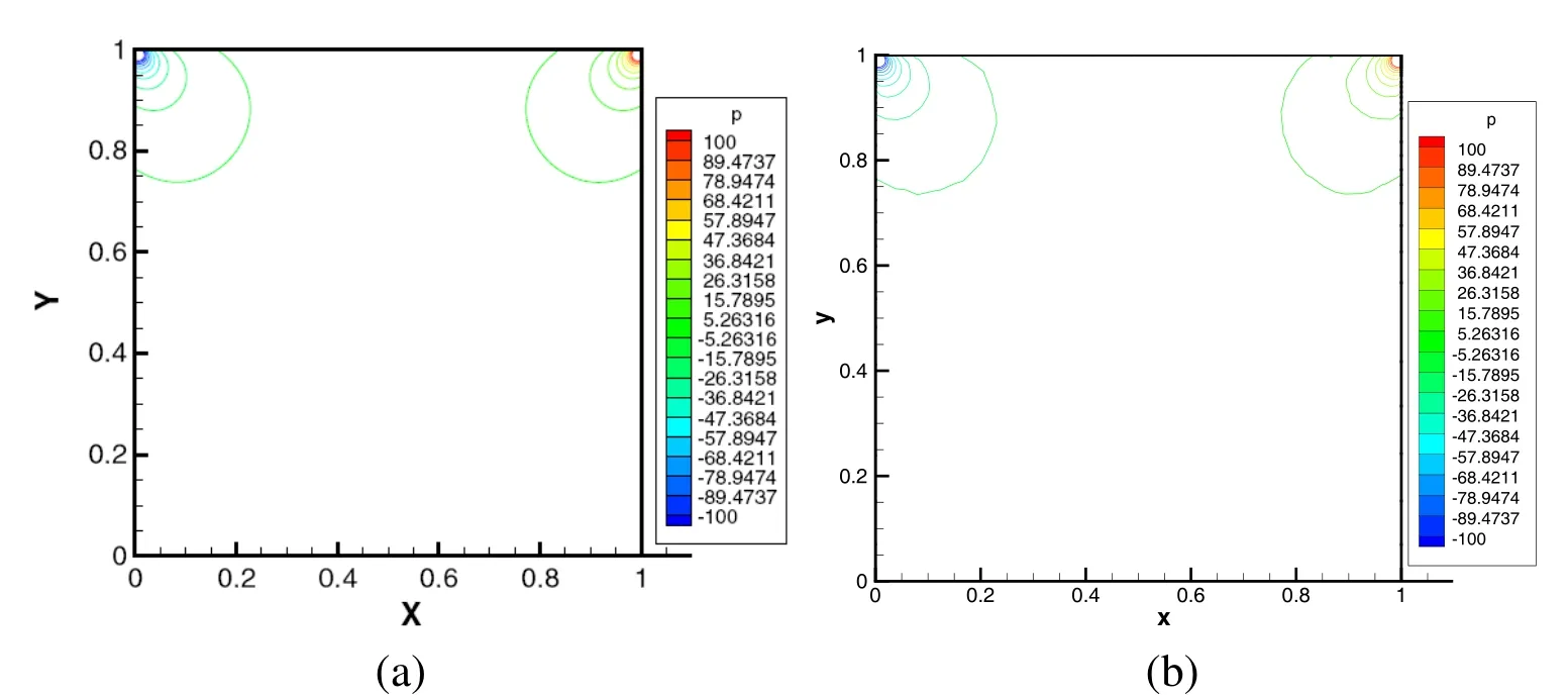
Figure 11:The pressure level lines:(a)with the Galerkin method on the much fine mesh in[Song,Hou,and Zheng(2013)]and(b)with the BLMG-based adaptive stabilized method.

4.4 The stokes flow over a step

The flow over a step is another benchmark problem which possesses the corner singularity.The computational domain is given by Ω =[0,4]× [0,1]−[1.2,1.6]×[0,0.4],and the flow is constrained with the Dirichlet boundary condition u=(0,0)at the upper and lower boundaries.Moreover,the in flow atx=0 is a parabolic flow u=(4y(1−y),0),whereas the out flow is a natural boundary condition.

Figure 12:From top to bottom:The initial mesh,the first adaptive mesh,and the second adaptive mesh.

Fig.12 shows the re fined meshes generated by the BLMG method based on the residual error estimator ηR.From Fig.12,the mesh refinement appears near the two corners of the step after several adaptive iterations.The related contour plots of the pressure based on these meshes are shown in Figs.13(a)-13(c).We can observe that numerical oscillation appears in the initial grid,while after enough adaptive iterations,the singular nature of the pressure is well captured with less oscillations.Meanwhile,the contour plot of the pressure based on uniform mesh using the Galerkin method(E=7205)is also shown in Fig.13(d),which is similar to that of the BLMG-based adaptive stabilized method(E=2533)given in Fig.13(c).This verifies again that our method can use less elements to achieve good results.

5 Conclusions

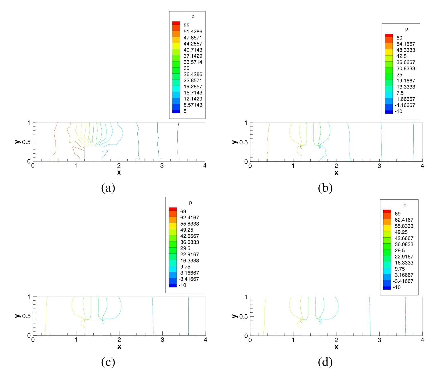
Figure 13:The pressure level lines on initial mesh (a), the first refined mesh (b)and the second refined mesh (c) using the BLMG-based adaptive stabilized method.The pressure level line on uniform mesh using the Galerkin method (d).

In this paper,we develop an adaptive node-based local mesh refining algorithm BLMG for the Stokes equations.Numerical tests show the efficiency and reliability of the adaptive BLMG method.The adaptive meshes generated by our method have good transition among elements,and the refinement or coarsening of the mesh in the adaptive process can be achieved at the same framwork through modifying the size function and controlling the node distribution.It also shows numerically that the BLMG-based adaptive stabilized method is very flexible which is independent of specific error estimators.Besides,since the satellite elements related to each central node are generated locally,the BLMG method has strong potential of parallelism,and the study of the parallel BLMG-based adaptive finite element method is our future work.

Acknowledgement:This research was supported by National Natural Science Foundation of China(Grant Nos:11471262,11471261,11101333),the Doctorate Foundation of Northwestern Polytechnical University(Grant No:CX201236),and NPU Foundation for Fundamental Research(Grant No:3102014JCQ01075).

Araya,R.;Barrenechea,G.R.;Poza,A.(2008): An adaptive stabilized finite element method for the generalized stokes problem.Journal of Computational and Applied Mathematics,vol.214,no.2,pp.457–479.

Arya,S.;Mount,D.M.;Netanyahu,N.S.;Silverman,R.;Wu,A.Y.(1998):An optimal algorithm for approximate nearest neighbor searching fixed dimensions.Journal of the ACM,vol.45,no.6,pp.891–923.

Babuvška,I.;Rheinboldt,W.C.(1978): Error estimates for adaptive finite element computations.SIAM Journal on Numerical Analysis,vol.15,no.4,pp.736–754.

Bank,R.E.;Welfert,B.D.(1990): A posteriori error estimates for the stokes equations:a comparison.Computer Methods in Applied Mechanics and Engineering,vol.82,no.1,pp.323–340.

Becker,R.;Braack,M.(2001):A finite element pressure gradient stabilization for the stokes equations based on local projections.Calcolo,vol.38,no.4,pp.173–199.

Biboulet,N.;Gravouil,A.;Dureisseix,D.;Lubrecht,A.;Combescure,A.(2013): An efficient linear elastic fem solver using automatic local grid refinement and accuracy control.Finite Elements in Analysis and Design,vol.68,pp.28–38.

Binev,P.;Dahmen,W.;DeVore,R.(2004): Adaptive finite element methods with convergence rates.Numerische Mathematik,vol.97,no.2,pp.219–268.

Bochev,P.B.;Dohrmann,C.R.;Gunzburger,M.D.(2006): Stabilization of low-order mixed finite elements for the stokes equations.SIAM Journal on Numerical Analysis,vol.44,no.1,pp.82–101.

Boussetta,R.;Coupez,T.;Fourment,L.(2006):Adaptive remeshing based on a posteriori error estimation for forging simulation.Computer Methods in Applied Mechanics and Engineering,vol.195,no.48–49,pp.6626–6645.

Chen,W.W.;Nie,Y.F.;Zhang,W.W.;Wang,L.(2012):A fast local mesh generation method about high-quality node set.Chinese Journal of Computational Mechanics,vol.29,no.5,pp.704–709.

Cuvelier,C.;Segal,A.;Van Steenhoven,A.A.(1986):Finite element methods and Navier-Stokes equations,volume 22.Springer.

Dohrmann,C.R.;Bochev,P.B.(2004): A stabilized finite element method for the stokes problem based on polynomial pressure projections.International Journal for Numerical Methods in Fluids,vol.46,no.2,pp.183–201.

Ervin,V.J.;Phillips,T.N.(2006): Residual a posteriori error estimator for a three- field model of a non-linear generalized stokes problem.Computer Methods in Applied Mechanics and Engineering,vol.195,no.19,pp.2599–2610.

Fujisawa,T.;Inaba,M.;Yagawa,G.(2003):Parallel computing of high-speed compressible flows using a node-based finite-element method.International Journal for Numerical Methods in Engineering,vol.58,no.3,pp.481–511.

He,Y.;Xie,C.;Zheng,H.(2010): A posteriori error estimate for stabilized low-order mixed fem for the stokes equations.Advances in Applied Mathematics and Mechanics,vol.2,no.6,pp.798–809.

Hecht,F.(1998):The mesh adapting software:bamg.inria report,1998.

Hecht,F.(2012):New development in freefem++.Journal of Numerical Mathematics,vol.20,no.3-4,pp.251–265.

Huang,Y.;Qin,H.;Wang,D.;Du,Q.(2011): Convergent Adaptive Finite Element Method Based on Centroidal Voronoi Tessellations and Superconvergence.Communications in Computational Physics,vol.10,no.2,pp.339–370.

Ju,L.;Gunzburger,M.;Zhao,W.(2006):Adaptive Finite Element Methods for Elliptic PDEs Based on Conforming Centroidal Voronoi-Delaunay Triangulations.SIAM Journal on Science Computing,vol.28,no.6,pp.2023–2053.

Kay,D.;Silvester,D.(1999): A posteriori error estimation for stabilized mixed approximations of the stokes equations.SIAM Journal on Scientific Computing,vol.21,no.4,pp.1321–1336.

Labergère,C.;Rassineux,A.A.;Saanouni,K.K.(2011): 2d adaptive mesh methodology for the simulation of metal forming processes with damage.International Journal of Material Forming,vol.4,no.3,pp.317–328.

Li,J.;He,Y.(2008): A stabilized finite element method based on two local gauss integrations for the stokes equations.Journal of Computational and Applied Mathematics,vol.214,no.1,pp.58–65.

Liao,Q.;Silvester,D.(2012): A simple yet effective a posteriori estimator for classical mixed approximation of stokes equations.Applied Numerical Mathematics,vol.62,no.9,pp.1242–1256.

Liu,Y.;Nie,Y.F.;Zhang,W.W.;Wang,L.(2010):Node placement method by bubble simulation and its application.CMES-Computer Modeling in Engineering&Sciences,vol.55,no.1,pp.89–109.

Morin,P.;Nochetto,R.H.;Siebert,K.G.(2000):Data oscillation and convergence of adaptive fem.SIAM Journal on Numerical Analysis,vol.38,no.2,pp.466–488.

Nicolas,G.;Fouquet,T.(2013):Adaptive mesh refinement for conformal hexahedral meshes.Finite Elements in Analysis and Design,vol.67,pp.1–12.

Nie,Y.F.;Chang,S.(2006): Node-based local mesh generation algorithm.Chinese Journal of Computational Mechanics,vol.23,no.2,pp.252–256.

Nie,Y.F.;Zhang,W.W.;Liu,Y.;Wang,L.(2010):A Node Placement Method with high quality for mesh generation.InIOP Conference Series:Materials Science and Engineering,volume 10,pg.012218.IOP Publishing.

Nie,Y.F.;Zhang,W.W.;Qi,N.;Li,Y.Q.(2014): Parallel node placement method by bubble simulation.Computer Physics Communications,vol.185,no.3,pp.798–808.

Nithiarasu,P.;Zienkiewicz,O.C.(2000): Adaptive mesh generation for fluid mechanics problems.International Journal for Numerical Methods in Engineering,vol.47,no.1-3,pp.629–662.

Picasso,M.(2003): An anisotropic error indicator based on zienkiewicz–zhu error estimator:Application to elliptic and parabolic problems.SIAM Journal on Scientific Computing,vol.24,no.4,pp.1328–1355.

Qi,N.;Nie,Y.F.;Zhang,W.W.(2014): Acceleration strategies based on an improved bubble packing method.Communications in Computational Physics,vol.16,no.1,pp.115–135.

Shewchuk,J.(2005):Triangle:A Two-Dimensional Quality Mesh Generator and Delaunay Triangulator.http://www.cs.cmu.edu/˜quake/triangle.html,2005.

Shimada,K.;Gossard,D.C.(1998):Automatic triangular mesh generation of trimmed parametric surfaces for finite element analysis.Computer Aided Geometric Design,vol.15,no.3,pp.199–222.

Song,L.;Hou,Y.;Zheng,H.(2013):Adaptive variational multiscale method for the stokes equations.International Journal for Numerical Methods in Fluids,vol.71,no.11,pp.1369–1381.

Verfürth,R.(1989):A posteriori error estimators for the stokes equations.Numerische Mathematik,vol.55,no.3,pp.309–325.

Verfürth,R.(1991):A posteriori error estimators for the stokes equations ii nonconforming discretizations.Numerische Mathematik,vol.60,no.1,pp.235–249.

Zhang,W.W.;Nie,Y.F.;Li,Y.Q.(2012): A new anisotropic local meshing method and its application in parametric surface triangulation.CMES-Computer Modeling in Engineering&Sciences,vol.88,no.6,pp.507–529.

Zheng,H.;Hou,Y.;Shi,F.(2010):A posteriori error estimates of stabilization of low-order mixed finite elements for incompressible flow.SIAM Journal on Scientific Computing,vol.32,no.3,pp.1346–1360.