
Numerical simulation of drag reduction characteristics for transverse groove pipeline*
2014-07-31 20:22LeleDUANSiyuSONGWangXIXiaoWEIYunboLIWeigangZHEN
机床与液压 2014年2期
Le-le DUAN,Si-yu SONG,Wang XI,Xiao WEI,Yun-bo LI,Wei-gang ZHEN
1School of Transportation, Wuhan University of Technology, Wuhan 430063, China;2Engineering Training Center,Wuhan University of Technology,Wuhan 430063,China
Numerical simulation of drag reduction characteristics for transverse groove pipeline*
Le-le DUAN†1,Si-yu SONG1,Wang XI1,Xiao WEI1,Yun-bo LI1,Wei-gang ZHEN†2
1SchoolofTransportation,WuhanUniversityofTechnology,Wuhan430063,China;2EngineeringTrainingCenter,WuhanUniversityofTechnology,Wuhan430063,China
In order to analyze the characteristics of the resistance in the transverse groove of pipelines, the standardk-εmodel was adopted to numerically calculate and compare the resistances under the conditions of different velocities in ten groups of pipelines, and the impact of speed and groove shape on the drag reduction could be obtained through these numerical simulations. Based on all these analysis, the drag reduction mechanism of groove pipelines could be obtained, i.e., the low-speed fluid is regarded as a layer of water film, which makes the high-speed fluid contacts with the inner wall of the tube, and the friction of the groove could be indirectly reduced. Therefore, the local fluid flow resistance will be decreased as the vortex zone within the groove becomes more regular.
Transverse grooves, Vortex zone, Drag reduction characteristics, Numerical simulation, Mechanism of drag reduction
1.Introduction
At the end of 1950s, Stanford has conducted a series of researches about turbulent boundary layer based on the flow field display technique. The following researches also show that the flow at the bottom of the viscous layer is different from the original concept and they further confirmed that the near-wall region has turbulence characteristics. All these researches guide scientists develop some surfaces to influence the fluid flow in the near-wall region of the turbulent boundary layer. Liu Kline and Johnson from Stanford tried this at the first time in 1966. From then on, many researches have been expanding based on the concept of ‘utilizing some unsmooth surface to reduce the frictional resistance’. In 1965, Kramer started to study the movements of dolphins which seemed as a start of researches on streak grooves. In 1967, Kiev hydrodynamics laboratory studied vortex screen and put forward the possibility of reduction in dynamics resistance on streak grooves. In 2005, Huang De-bin used numerical simulation to study the drag reduction on turbulence in the groove of pipelines and gained the same results from the grooves of planks[1]. Lee and Jang pasted V-grooves on NACA 0012 airfoil section and found that the resistance of rear airfoil was reduced by 6.6%[2-3].
In the real pipelines, head loss contains frictional loss and local resistance loss. The transverse grooves will increase the local resistance, at the same time, the friction loss could be reduced. This paper analyzed the drag reduction of different place to smoothing in grooves by using the Fluent software.
2.Numerical computation methods
2.1.Objects description
There are ten types of rotation faces for pipelines, as shown in Figure 1. The pipe diameter is 8 mm, pipe range is 23 mm, groove height is 2 mm, groove range is 3 mm, and the radius of transitional curve is 1 mm. The turning points of the different parts are named as the number 1, 2, 3 and 4, as shown in Figure 1. The groove represents the transverse groove without transitional curve. Since it is centrosymmetric periodic flow in the pipes, the revolution surfaces will be studied and the corresponding grids are shown in Figure 2.

Figure 1. Pipe model

Figure 2. Schematic diagram of grid
2.2.Numerical model
Since the steady state centrosymmetric incompressible flow in pipes will be studied in this paper, the continuity equation of three-dimensional incompressible fluid flow is as follows.
Where,ux,uy,uzare the velocity components inx,yandzdirection, respectively. The variable oftis time.
Conservation of momentum equations for incompressible fluid flow could be obtained as follows.
The standardk-εmodel is adopted as turbulent model.
Where,kis the power of turbulence,Eis the dissipation rating, andCL=0.09,C1ε=1.44,C2ε=1.92,Rk=1.0.
2.3.Boundary conditions
According to the Fluent software, the solver could be chosen as Pressure-Based type, steady state, non-slip wall boundary and 2D axisymmetric swirl flow. The viscous model is standard k-ε model and the standard Wall Function is applied. The fluid material is liquid water and inlet velocities are 1.0 m/s, 2.0 m/s, 4.0 m/s, 6.0 m/s, 8.0 m/s and 10 m/s respectively.
The velocity-inlet boundary is applied in this paper and the The entrance is velocity-inlet,velocity specification method is magnitude/normal to boundary, the exit boundary is outflow.
3.Analysis of numerical simulation results
3.1.Relationships between pressure drag and velocity
The relationships between pressure drag and velocity are shown in Figure 3. Since the pressure drag of straight pipe is the reference value, it is set as zero. From this figure, it could be seen that the pressure drags of other pipes are increased as the increase of inlet velocity. When the inlet velocity is small, the values of pressure drag for all these pipes are very close. However, once the inlet velocity is beyond 6 m/s, place1 has the max pressure drag while the place 3 and place 4 have the minimum values.

Figure 3. Pressure drags in different velocities
3.2.Frictional drag with different velocities
As shown in Figure 4, the frictional drag in straight pipe is increased faster than that in the pipes with grooves when the inlet velocity gets increased. However, all the pipes with groove have nearly the same increase in terms of frictional drag and the flow resistance mainly depends on pressure drags. Therefore, in order to reduce the flow resistance in pipes when velocity is high, the pressure drags need to be reduced.

Figure 4. Frictional drag in different velocities
3.3.Total resistance with different velocities
As shown in Figure 5, the relationships between total resistance and velocity are presented. The total resistance is defined as the summation of pressure drag and frictional drag. From this figure, it could be seen that the total resistances of different pipes have almost the same growth rate with the increase of velocity. However, with the increase of velocity, the minimum flow resistance is changed for different types of grooves. When the velocity is below 3.3 m/s, the square shaped groove has the minimum resistance. When the velocity reaches up to 4 m/s, pipes with 34 smoothing have the minimum resistances.
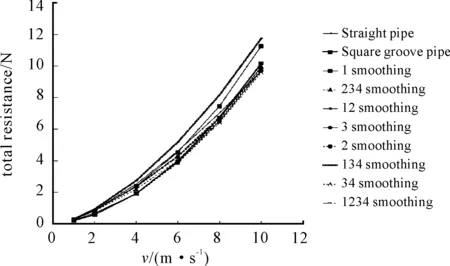
Figure 5. Total resistance in different velocities
4.Analyzing of drag reduction efficiency
Figure 6 shows the differences between straight pipes and groove pipes under the conditions of different velocities. Figure 7 shows the drag reduction efficiency in different types of grooves.
DFi=Fz-Fi
Drag reduction efficiency is defined as follows:
▯=DFi/Fz
Where,Fzis the total resistance in straight pipe,Fiis the total resistance in different types of grooves.
From the Figure 6, it could be seen that the grooves with 134 smoothing have no drag reduction. The higher the velocity is, the faster the total resistance increase. When velocity reaches up to 6 m/s, most pipes have best efficiencies; however, when velocity is beyond 9 m/s, straight pipes have minimum resistance among all these pipes and other pipes have no drag reduction when the velocity is up to 10 m/s.
It could be seen in Figure 7, when velocity is 2 m/s, the square grooves have the best drag reduction at 33%. Once the velocity is below 4 m/s, most of the drag reduction efficiencies in various types will increase alone with the velocity. When the velocity is higher than 4 m/s, the drag reduction efficiencies of all these various types will decrease as the increase of velocity. The grooves with 34 smoothing have the best drag reduction. When velocity is 4 m/s, the drag reduction efficiency is 21.63%.

Figure 6. Drag reduction in straight pipes and grooves pipes in different velocities

Figure 7. Drag reduction efficiency in different types of grooves
5.Analysis of drag reduction mechanism
Since the existence of grooves within pipe makes the fluid velocity become slow and they work as water film which could force the fluid contact with the tube wall indirectly, the frictional resistance will be reduced. Meanwhile, as shown in Figure 8 and Figure 9, the turbulence area has been moved back due to the existence of grooves and the Fluid becomes steady both in front of the groove and behind the grooves. Therefore, the turbulence area has almost gone. When the grooves are optimized, the decrement of the frictional resistance is greater than the increment of pressure resistance. When the velocity is small, the vortex becomes nearly static due to the arise of the square grooves, as there is only a large regular vortex movement in the groove, as a result, most wetted surface is at a small velocity region and the frictional resistance is within a small range. As shown in Figure 10 and Figure 11, those transitional curves make the wetted surface larger and the vortex becomes irregular so that the local resistance gets increased.

Figure 8. Velocity vector in square groove

Figure 9. Velocity vector in straight pipe

Figure 10. Velocity vector in square groove

Figure 11. Velocity vector in 134 smoothing groove
6.Conclusion
Within a relative big velocity range, i.e., from 1.0 m/s to 10.0 m/s, the numerical simulations are adopted to analyze the pressure resistance, frictional resistance and total resistance for ten types of grooves within pipes in this paper, and the efficiency of those pipes are evaluated as compared with that of straight pipes. The conclusions could be drawn as follows:
1) Grooves in straight pipes could make turbulence area move back to reduce frictional resistance and fluid flow in grooves is at a relative low velocity, therefore the frictional resistance is at a low degree. Local resistance increases alone with the increase of velocity so that the drag reduction efficiency is low. When velocity reaches up to 10 m/s, the fluid flow resistance will be increased.
2) The shape of the grooves has dominant effects on the fluid flow resistance. Different grooves have different levels of regular vortex. The more regular the vortex is, the less the resistance is. When velocity is small, the fluid in square groove works as a water film separating the fluid from the tube wall and the fluid flow resistance could be reduced. However, those transitional curves make the fluid and wall contact well, and the frictional resistance could be increased.
3) Different velocities correspond to different optimal shapes of grooves. As a result, different shapes of grooves should be adopted for different values of velocity.
[1] Guo X.Optimization Design Method For Drag reduction Over Riblet Structure[D].Xi’an:Northwest Polytechnic University,2007.
[2] Huang D,Deng X,Wang Y.Numerical Simulation Study Of Turbulent Drag Reduction Over Riblet Surfaces Of Tubes[J].Journal Of Hydrodynamics,2005.
[3] Lee S,Jan Y.Control of flow around a NACA0012 airfoil with a micro-riblet film[J].Journal of Fluids and Structures,2005.
横向凹槽管道的减阻特性数值模拟研究*
段乐乐1,宋思宇1,奚 望1,魏 骁1,李云波1,郑卫刚2
1.武汉理工大学 交通学院,武汉 430063;2.武汉理工大学 工程训练中心,武汉 430063
针对管道内横向凹槽减阻问题,采用标准κ-ε模型,通过数值仿真,计算比较了在10组管道内不同流速情况下的阻力,分析了速度和凹槽形状对减阻的影响。得到凹槽减阻机理:凹槽内的低速流体相当于一层水膜,可使高速流体不直接与管内壁接触,从而减小摩擦阻力;同时凹槽内漩涡区越规则,局部阻力越小。
横向凹槽;漩涡区;减阻特性;数值仿真;减阻机理
TQ022.1
2014-02-01
10.3969/j.issn.1001-3881.2014.12.011
*Project supported by National Undergraduate Training Programs for Innovation and Entrepreneurship(20131049702002)
† Wei-gang ZHEN. E-mail: zfeidiao@126.com
猜你喜欢
橡塑技术与装备(2021年6期)2021-03-19
武汉理工大学学报(交通科学与工程版)(2019年4期)2019-08-29
武汉理工大学学报(信息与管理工程版)(2019年3期)2019-07-15
武汉理工大学学报(交通科学与工程版)(2019年3期)2019-07-02
汽车观察(2018年10期)2018-11-06
制造技术与机床(2018年10期)2018-10-13
中外文摘(2017年19期)2017-10-10
中国铸造装备与技术(2017年3期)2017-06-21
中国卫生(2016年4期)2016-11-12
设计艺术研究(2015年4期)2015-06-28

- 机床与液压的其它文章
- A Simple time-domain method for bearing performance degradation assessment*
- Structural design and performance testing of the electromagnetic proportional pressure relief valve
- Analysis of magnetic field characteristics for different winding cylinder materials of a new type of magnetorheo-logical damper*
- Impacts of centrifuge errors on calibration accuracy of error model coefficients of gyro accelerometer*
- Interior ballistic simulation and parameter influence analysis of an underwater pneumatic launcher*
- Influence of airflow uniformity over the duct outlet of vehicle air-condition on cooling performance*