Equipment Maintenance Material Demand Forecasting Based on Gray-Markov Model

BI Kun-peng(毕坤鹏), ZHANG Hong-yuan(张宏运), YAN Guo-hui(晏国辉), TANG Na(唐 娜)

1 Chemical Defense Equipment Department,Institute of NBC Defense of PLA, Beijing 102205, China 2 Biological and Chemical Defense Department, Institute of NBC Defense of PLA, Beijing 102205, China

Equipment Maintenance Material Demand Forecasting Based on Gray-Markov Model

BI Kun-peng(毕坤鹏)1*, ZHANG Hong-yuan(张宏运)1, YAN Guo-hui(晏国辉)1, TANG Na(唐 娜)2

1ChemicalDefenseEquipmentDepartment,InstituteofNBCDefenseofPLA,Beijing102205,China2BiologicalandChemicalDefenseDepartment,InstituteofNBCDefenseofPLA,Beijing102205,China

Maintenance material reserves must keep an appropriate scale, in order to meet the possible demand of support objectives. According to the sequence of maintenance material consumption, this paper establishes a Gray-Markov forecasting model by combining Gray system theory and Markov model. Few data are needed in the proposed Gray-Markov forecasting model which has high prediction precision by involving small parameters. The performance of Gray-Markov forecasting model was demonstrated using practical application and the model was proved to be a valid and accurate forecasting method. This Gray-Markov forecasting model can provide reference for making material demand plan and determining maintenance material reserves.

maintenancematerial;gray-Markov;demandforecasting;materialreserves

Introduction

The demand quantity of maintenance material is the main proof for making material support plan and determining the reserves. Precise forecasting for maintenance material demand quantity is convenient to establish material support plan and determine material reserves, and can improve material quality and further benefit material support. Currently, equipment maintenance material demand forecasting is mainly dependent on experience and history data, and lacks scientific and exact forecasting methods. The theory of gray system is founded by Professor Deng Julong in 1982, which is a new method for uncertainty problems with few data and deficient information. Forecasting based on Gray model requires few data, which doesn’t require data following typical probability distribution and is fit for short period forecasting with better precision[1]. However, it is not fit for long period forecasting because the model could not calculate random fluctuation trend[2]. Many literatures indicate that different forecasting model has its respective advantages and disadvantages, and these methods are correlative and complementary for each other[3]. Markov forecasting method is a kind of forecasting method which can calculate the probability of occurrence for events with some sequence. Markov model is fit for time sequence forecasting with bigger random fluctuation character, and can macroscopically depict the whole change trend of time sequence[4-5]. The article develops a Gray-Markov forecasting model, which combines gray system theory and Markov theory[6], forecasts material demand based on the maintenance material wastage history data, and provides definite reference for maintenance material reserves.

1 Forecasting Model Basic Thought

Making use of gray model posts development change trend of maintenance material history wastage data, make sure state transfer on maintenance material wastage in the future period of time combining Markov forecasting means, and make sure wastage by use of state transfer.

Idiographic steps are: (1) make use of gray GM(1, 1) model process mimesis on equipment maintenance material history wastage data and compute mimesis error between GM (1, 1) model mimesis value and actual value; (2) process state partition according to Markov forecasting state partition means and acquire warp orderliness of mimesis error; (3) compute state transfer of mimesis error in the future forecasting time and make sure mimesis error size according to state transfer; (4) make Markov amend on mimesis result of GM(1, 1) model combing state partition means.

2 Gray-Markov Forecasting Model

2.1 Constitution of GM(1, 1) model

The parenchyma of constitution GM (1, 1) model is to make an accumulative addition for original data in order to take on definite orderliness, and acquires mimesis curve for system forecasting through constituting differential equation model[7-9]. The process is as follows.

Step 1:data making

According to original data sequence,

(1)

Make once data generating, and get data making sequence,

(2)

(3)

Step 2:data matrix constitution

Constitute data matrix, namely coefficient matrixBand original data sequence vectorYN:

(4)

(5)

Step 3: calculation parameter

(6)

Step 4: constitution gray model

Calculation differential equation:

e=2.718.

(7)

Step 5:calculation forecasting value

The forecasting value is:

(8)

2.2 Compartmentalization Markov state

Compartmentalization state is the key step in Markov forecasting. The mimesis errorΔ(i) between mimesis value and actual value is the system object. Generally, when original data quantity is less, subarea should be less so as to increase transfer time between all kinds of states and more impersonally reflect transfer orderliness between all kinds of states. When original data quantity become more, subarea should be more in order to dig more information from history data and increase forecasting precision[10-11]. CompartmentalizingΔ(i) tomstates, any state is:

(9)

whereEiis theith state;Δ1(i) andΔ2(i) are respectively the upper and lower limits ofEistate.

2.3 Calculation state transfer probability matrix

If current system is the state ofEi, we can calculate relevant probabilities of the system in all kinds of states through calculating state transfer probability matrix. Givenpi jis one step transfer probability of the system fromEistate toEjstate[12-13],

(10)

whereMiis the amount inEistate,Mi jis the amount of the system fromEistate toEjstate by one step, and we can achieve one step transfer probability matrixp(1)from state sequenceEi.

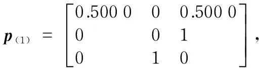
(11)

Calculate multi-step state transfer probability matrix according to Chapman-Kolmogorov equation.

(12)

2.4 Confirming system state transfer

Selectttimes away from forecasting time, and the transfer steps from near time to far time are respectively 1, 2, …,t. If the system state vector denotesCkinkth time away from forecasting time, then the state transfer probability matrix isp(k), andS(k)denotes state transfer probability matrix byksteps state transfer from the state[14],

S(k)=Ckp(k)=(p(k1),p(k2), …,p(ki), …,p(km)).

(13)

2.5 Forecasting result calculation

After making sure the system state transfer, we can compute Gray-Markov forecasting value through amending the error of gray mimesis value by use of median value in the subarea of system state[15],

(14)

3 Case Analysis

The paper considers year demand quantity of certain type equipment maintenance material, counter tube, as the research object. The material belongs to electronic component type, whose year wastage history data are less. Given the influences of inhesion attribute and by using intensity, management leveletc. factors, wastage data take on larger undulation character. Gray-Markov forecasting model is suitable for forecassting wastage statistics. According to actual investigation, the actual wastage of certain type of equipment maintenance material from year 2009 to 2013 is shown in Table 1.

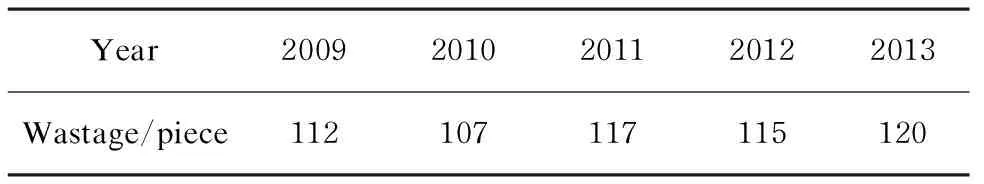
Table 1 Certain type of counter tube year wastage statistics

3.1 Calculation of gray forecasting value

Time response equation of gray GM (1, 1) model by calculating is

4398.6e0.024 3k-4283.6.

(15)

Calculate forecasting value,

(16)

Forecast demand quantity, namely forecasting value whenk=5,

(17)

The maintenance material gray forecasting value and actual value are shown in Fig.1.

Fig.1 Comparison of the gray forecasting value and actual value

3.2 Compartmentalization Markov state

After calculating mimesis errorΔ(i) , we can establish state partition table according to error. The least value is the lower limit, and the largest value is the upper limit. Error range of any corresponding results can be shown in Table 2. Then we can make state partition combine mimesis error, as shown in Table 3.

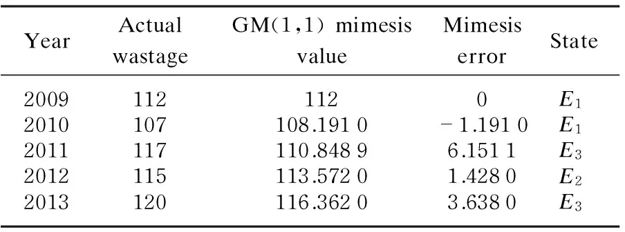
Table 2 Certain type equipment materialactual wastage and GM(1,1) mimesis value

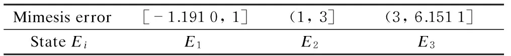
Table 3 Error range and state partition

3.3 Calculating state transfer probability matrix

(18)

According to state transfer probability formula, we can calculate state transfer probability matrices by 2-4 steps state transfer in turn, as follows,

(19)

(20)

(21)

3.4 Confirming state transfer

The transfer step of the nearest four years from near time to far time away forecasting time 2014 year is respectively 1, 2, 3, and 4. The system is on the state ofE3in 2013 year. Here system state vector denotesC1=(0 0 1), one step transfer probability from 2013 is:

S1=C1·p(1)=(0 1 0).

(22)

In common, calculate state transfer probability by 2-4 steps, and establish transfer probability table, as shown in Table 4.

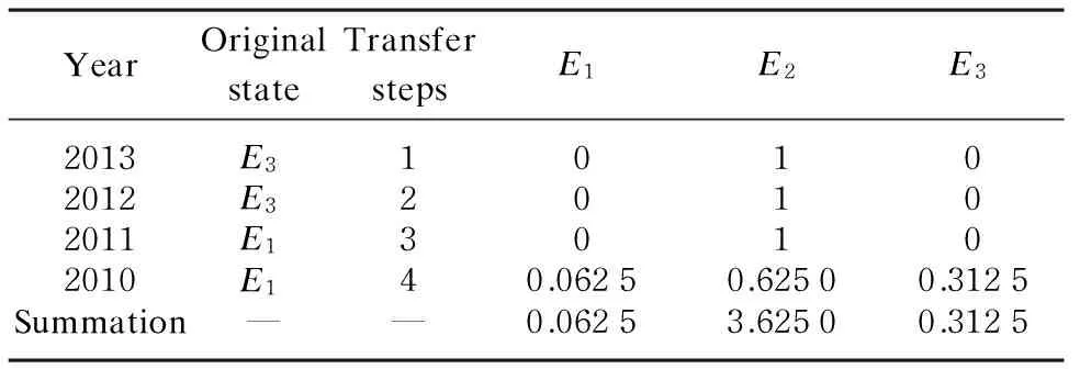
Table 4 Transfer probability of mimesis error Δ(i) in 2014

From Table 4 the largest accumulative probability is 3.6250. So, system state will transfer fromE3toE3.

3.5 Calculation of forecasting result

The forecasting wastage of certain type equipment maintenance material is 119.23 according to gray GM (1, 1) model in 2014. The forecasting wastage of certain type equipment maintenance material according to gray-Markov combination forecasting model is:

123.8153.

The forecasting integral wastage is 124 pieces.

3.6 Comparison and analysis about history data forecasting error

For checking up the forecasting precision of gray-Markov forecasting model, we contrast gray-Markov forecasting value with gray forecasting value, as shown in Table 5.

Table 5 Error ratio comparison between the actual value and the forecasting value

GM(1, 1)-forecasting value, GM(1, 1)-Markov forecasting value, and actual value of the certain type equipment maintenance material are shown in Fig.2.

The average mimesis error is 2.69% only by use of gray GM(1, 1) forecasting model in Table 5. However the average mimesis error is 0.91% by use of gray GM(1, 1)-Markov combination forecasting model. For time sequence forecasting with less history data and larger random undulation character, Table 5 reflects that GM(1, 1)-Markov can increase precision and reliability of forecasting compared with singleness gray forecasting model. Gray-Markov model can satisfy the need of electronic component type maintenance material wastage forecasting.

Fig.2 Comparison between the gray-Markov forecasting value and the actual value

4 Conclusions

A GM(1,1)-Markov combination forecasting model is developed by combining the advantage in trend of gray forecasting and the advantage in integral fluctuation sequence of Markov forecasting, and proved that it has higher forecasting precision compared with single forecasting model. The establishment course of combination forecasting model is simple, which can be implemented through program. At the same time, the model can be improved in real time based on the maintenance material history data variety. The forecasting model can provide an important foundation for scientifically forecasting maintenance material demand quantity and ascertaining material reserves quantity reasonably.

[1] Liu S F, Xie N F. Gray System Theory and Application [M]. Beijing: Beijing Science Press, 2008: 1-10. (in Chinese)

[2] H J X, H Z X. Gray Control [M]. Beijing: National Defense Press, 2005: 13-36. (in Chinese)

[3] Wang T S, Zhang T. Combining Forecasting-Theory, Method and Application [M]. Beijing: Beijing Social Science Document Press, 2008: 30-50. (in Chinese)

[4] Chen Y H. Combining Forecasting Method Effectiveness Theory and Application [M]. Beijing: Science Press, 2008: 1-15. (in Chinese)

[5] Zheng X P. Accident Forecasting Theory and Method [M]. Beijing: Tinghua University Press, 2010: 120-180. (in Chinese)

[6] Tong C S. Introduction to the Theory and Method on Systems Engineering [M]. Beijing: National Defense Press, 2005: 165-166. (in Chinese)

[7] Zhang W, Deng Y C. Short Term Wind Speed and Wind Electricity Power Forecasting Based on Gray-Markov Chain [J].ElectricPower, 2013, 46(2): 98-102. (in Chinese)

[8] Cui H, Zhu X M, Teng L. Plough Forecasting Based on Gray-Markov Model in Jinan City [J].LandandResourcesinShandongProvince, 2013, 29(2): 42-45, 89. (in Chinese)

[9] Liu X G, Zhou B Y. Road Freight Demand Forecast Based on Gray-Markov Relation [J].CentralSouthHighwayShandong, 2013, 38(1): 111-113. (in Chinese)

[10] Liu W C, Chen T. To-and-fro Pump State Scout and Trend Forecasting Based on Gray-Network [J].JournalofSafetyScienceandTechnology, 2013, 9(1): 79-84. (in Chinese)

[11] Li C. Combinatorial Forecasting of Logistics Volume of Shanghai Based on Gray Neural Network [J].LogisticsTechnology, 2013, 32(1): 143-146. (in Chinese)

[12] Du J L, Wang L, Zhang J F,etal. Application on Vehicle Maintenance Material Demand Forecasting Based on Gray System Theory [J].LogisticsTechnology, 2009, 28(11): 249-251. (in Chinese)

[13] Liu P, Miao Y J, Zhang J J. Prediction of Gear Life Based on Grey-Markov Model [J].CoalMineMachinery, 2010, 31(9): 51-53. (in Chinese)

[14] Zhang C, Zhang K S. Forecasting on Railway Freight Volume Based on Gray-Markov Chain Model [J].TechnologyandMethod, 2011, 30(7): 129-133. (in Chinese)

[15] Li B M. The Armed Police Logistics War Material Demand Forecasting Based on Gray Markov Model [J].JournalofEngineeringUniversityofCAPF, 2013, 29(2): 51-55. (in Chinese)

Foundation item: Chemical Defense Equipment Maintenance Material Support Methods, Universal Equipment Support Department [2012] No.80, China

1672-5220(2014)06-0824-03

Received date: 2014-08-08

* Correspondence should be addressed to BI Kun-peng, E-mail: ikunpeng@sina.com

CLC number: E23 Documet code: A