REGULARITY FOR A GENERALIZED JEFFREY’S INTEGRAL MODEL FOR VISCOELASTIC FLUIDS∗

Department of Numerical Mathematics,Faculty of Mathematics and Physics, Charles University in Prague,Sokolovsk´a 83,Praha 6,186 75,Czech E-mail:soukup@karlin.mf.cuni.cz

REGULARITY FOR A GENERALIZED JEFFREY’S INTEGRAL MODEL FOR VISCOELASTIC FLUIDS∗

Ivan SOUKUP

Department of Numerical Mathematics,Faculty of Mathematics and Physics, Charles University in Prague,Sokolovsk´a 83,Praha 6,186 75,Czech E-mail:soukup@karlin.mf.cuni.cz

We prove a local existence of a strong solution v:Ω×T→R3for a system of nonlinear integrodiferential equations describing motion of an incompressible viscoelastic fuid using standard mathematical tools.The problem is considered in a bounded,smooth domain Ω⊂R3with a Dirichlet boundary condition and a standard initial condition.

integral model;viscoelastic fuid;strong solution

2010 MR Subject Classifcation76A10;45K05;45G10

1 Introduction

Let Ω⊂R3be an open,bounded set and T＞0.We denote QT:=Ω×(0,T).We are interested in a local existence of a strong solution to the following system of equations

Remark 1.1It is well known([12])that the motion of an incompressible fuid with constant density ρ is in an isothermal case governed by the system of equations

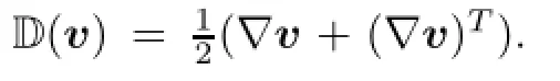
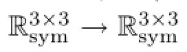
and without loss of generality,we consider the density ρ to be equal to 1.Let us emphasize that obviously the stress tensor S is not linked with D in a point-wise manner as it is usual.

1.1 Preliminaries

Remark 1.2Since we are interested only in the behaviour of velocity at positive times, we assume without loss of generality that v≡0 on(-∞,0)×Ω.This assumption,together with(1.8)yields

Remark 1.3The model that we have just introduced represents a theoretical generalization of Jefrey’s integral model for viscoelastic fuids.

we denote the Bochner spaces.For p≥1 we defne

1.2 Mathematical Formulation of the Problem

At this point we present a precise mathematical formulation of the problem given by system (1.1)complemented by the Dirichlet boundary condition and the initial condition.

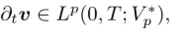
Defnition 1.4(Problem P)Let Ω∈ℭ3,T＞0 and p＞1.Assume that f∈L2(0,T;L2(Ω)3)and v0∈Vpare given.Find(v,π)such that

Before we introduce the notions of weak and strong solutions to the Problem P let us mention that assumption(1.4)implies the symmetry of F while the assumption(1.7)implies the symmetry of H.

Defnition 1.5(Weak solution)We call a function v a weak solution of Problem P if and only if the following conditions are satisfed:

·the weak formulation

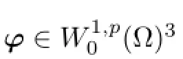
holds for all φ∈Vpand almost every t∈[0,T],

Defnition 1.6(Strong solution)We call a couple(v,π)a strong solution of Problem P if and only if the following conditions are satisfed:

1.3 Main Result

The purpose of this paper is to provide a new result about regularity of solution to the presented mathematical problem by means of standard mathematical tools and approaches. The main result is summarized in the following theorem.

holds and

2.We would also like to mention another known papers studying model without memory term that in our opinion present methods which might be applicable to our problem.Wolf [23]has extended the existence results of Ladyzhenskaya to p≥8/5 without any additional assumptions.Also,the results from Diening,R˚uˇziˇcka,Wolf[7]extended the existence results without any additional assumptions on F even for p≥6/5.Furthermore,if one can successfully adopt methods from[5]and prove time regularity of solution,then it should be elementary to apply the procedure from[6]and extend the regularity results.Also,paper by Bae and Wolf[3] can extend the regularity results if one can overcome the complications arising from point-wise approach in[3](see Section 3 therein).One way we can look at procedures presented in those papers is based on the last sentence of Remark 1.1.We work on a more general setting where we do not have a point-wise behaviour of the Cauchy stress tensor.This represents the maindiference between our problem and the problem studied in papers mentioned in this paragraph.

3.Equations similar to(1.9)were studied by Agranovich and Sobolevskii(see[1,2]).In[2] a local in time solution was obtained in a three-dimensional space under assumptions on F and H that difer from ours in many aspects(the forms F and H depend on the second invariant of symmetric part of velocity gradient and satisfy rather restrictive boundedness conditions,but do not need so strong monotonicity).

4.There exist several papers that study the presented system with an additional integral equation describing past motions of a particle and a memory term depending on its trajectory. In papers by Dmitrienko,Vorotnikov and Zvyagin([8,9]and[22])the existence of weak solutions for the linear forms F and H was proven.Orlov and Sobolevskii[19]proved even local existence and uniqueness of strong solution in the case of linear F.Nevertheless,we are more interested in models with non-linear operator F and memory depending directly on symmetric gradient of velocity.

5.We follow the method used in M´alek,Neˇcas,R˚uˇziˇcka[17]in order to prove the regularity results formulated in Theorem 1.7.We will concentrate our future eforts on extending the existence results using methods from[23]and[7].

6.Let us outline the main parts of the proof of the main result.In the following chapter we formulate the approximate problem to the Problem P.The third chapter focuses on the proof of the existence of a strong solution to the approximate problem based on the classical Nirenberg translation method.The forth and ffth chapter deal with the limit passage.

2 Defnition of the Approximate Problem

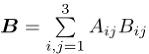
Lemma 2.1(originally in[4],Lemma 2.1)Let H and G satisfy corresponding assumptions (1.7)-(1.8).Then for all φ∈L2(0,T;(L2(Ω))3×3)symmetric holds an inequality

The following lemma is analogous to[16],Chapter 5,Lemma 1.19 and Lemma 1.35.We refer to the aforementioned paper for the proofs.

It is well-known that

and it is easy to show that the mollifcation of v also satisfes

where c is a constant independent of ε.For the sake of completeness let us mention an obvious observation that if divv=0 then divΠεv=0.

Now,we redefne our problem with mollifed convective term.We will denote this modifed problem as Problem Pε.

Defnition 2.3(Problem Pε)For given ε＞0 fnd(v,π)=(vε,πε)such that

We cannot obtain this estimate for all t∈[0,T]and this is partly the reason why we are able to prove regularity only locally in time(see Theorem 1.7).In the end of this paper we show why we cannot extend the solution on the whole time interval[0,T]as it is done in the case of existence result by B´arta in[4].

Moreover,since∂tv is not admissible test function in weak formulation,we derive the following a priori estimate at least formally.We multiply(2.8)by∂tv(which is also divergencefree and vanishing at∂Ω),integrate over Qtand use the identity

along with Lemma 2.2 to get

Lemma 2.4Let v∈L∞(0,T;H)∩L2(0,T;V2).Then for any ε＞0 and for all t∈[0,T]

where c∞is positive constant from embedding W2,2→L∞.

ProofWe compute

Finally,in order to obtain higher regularity properties we need more information about∇v. Thus,we want to,at least formally,derive a priori estimate that will give us such information. We cannot use-Δv as a test function because it does not vanish at the boundary(although it is divergence-free).Thus,we solve this problem using a so-called cut-offunction.

From Defnition 2.6 it is easy to observe that FAhas linear growth(see the inequality (2.19)1below)and divFA(D(·))maps L2(0,T;V2)→L2(0,T;V∗2).Thus we fnally come to the defnition of the approximate problem.

·the weak formulation

holds for all φ∈V2and almost every t∈[0,T∗],

·the weak formulation

Remark 2.10A strong solution(v,π)satisfy the equation(2.16)almost everywhere in QT∗thanks to the linear growth of FAand H and the regularity properties of strong solution.

ProofFirst the lipschitzity follows easily from(2.19)2

Second,the monotonicity follows immediately from(2.21)

3 Strong Solution to Approximate Problem

where cnegis the constant from Theorem 7.4.The necessity of these restrictions will be justifed in the rest of the paper.

and the equation(2.16)holds almost everywhere in QT∗(see Remark 2.10).

The proof of Theorem 3.1 consists of two main parts.First,we prove the existence of a weak solution along with the estimates(3.2)and(3.3)using Galerkin approximations and monotone operator theory.Also,we show the estimate(3.4)holds as a consequence.Second, we prove the regularity estimate(3.5)using the methods from[17].

3.1 Existence of Galerkin Approximations

with initial condition ci(0)=ai.

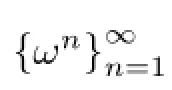
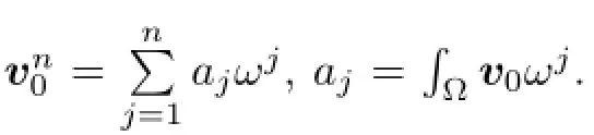
ProofFirst,for c:=(c1,···,cn)∈Rnand ω:=(ω1,···,ωn)∈(Vn)nwe denote

where a=(a1,···,an)is the initial condition and χ denotes the characteristic function.After integrating from 0 to t and using Fubini’s theorem,(3.7)yields

In the next section we show that vn∈L∞(0,T∗;H)which implies that our solution c to(3.7)is defned on the whole R+.We will call the functions vn(t,x)the n-th Galerkin approximation.

3.2 A priori Estimates

We show the following a priori estimates for the Galerkin approximations

Lemma 3.3Let vn,n=1,2,···,be the n-th Galerkin approximation defned in Section 3.1.Then for all t∈[0,T∗]holds

ProofWe multiply(3.6)by ci(s),sum over i and integrate over(0,t)(notice that divvn= 0 so the term containing pressure vanishes).Namely we have

Thanks to the Young’s and H¨older’s inequalities along with properties of FAand H we have

where Cyis a positive constant from Young’s inequality.Finally,using Korn’s inequality(7.1) and plugging the term U into the left-hand side we obtain

Lemma 3.4Let vn,n=1,2,···,be the n-th Galerkin approximation defned in Section 3.1.Then for all t∈[0,T∗]holds

Now we estimate each term in(3.14)separately

Using Green’s theorem(frst in spatial then in time variable)we get

Using identity(2.10)which is permissible for Galerkin approximations,we have

Moreover,from the inequality(2.20)follows that

We fnally get the estimate

which clearly leads to the desired conclusion. ?

3.3Convergence of Galerkin Approximations

ProofThe validity of the frst three limits can be shown in a standard way.Consequently, the rest follows from compact embeddings theory of Sobolev spaces and properties of Bochner spaces.?

In order to make a limit passage for n→∞,we multiply the equation(3.6)by a function ψ∈D(0,T∗)and integrate over(0,T∗).We obtain

thanks to the convergence properties(3.15),regularity properties of the mollifcation function and Sobolev embeddings.

The remaining terms are treated in the following way.

Lemma 3.6Defne for a.e.(x,s)∈QT∗and all n∈N function

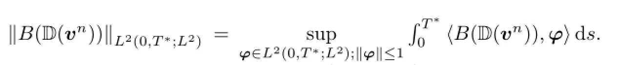
Then B(D(vn))is bounded in L2(0,T∗;L2)independently of n.

Therefore,there exists~B∈L2(0,T∗;L2)such that B(D(vn))⇀~B in L2(0,T∗;L2).The limit passage for n→∞will be complete if we show that for allφ∈L2(0,T∗;V2)and a.e. t∈(0,T∗)

Let us assume that for allφ∈L2(0,T∗;V2)and for all ε∈R

Then,using the lipschitzity of FAand H(we denote λBas the lipschitz coefcient for B),we have

which holds for all ε∈(-δ,δ)and for φ as well as for-φ.This implies

3.4 Reconstructing the Pressure

If we defne

Thus the frst part of the proof of Theorem 3.1 is complete.

3.5 Regularity Estimate

Now,we prove the regularity estimate(3.5)having at our disposal the estimates(3.2), (3.3)and(3.4)and the weak formulation(2.18).We will continue the proof using the classical Nirenberg translation technique analogously as in M´alek,Neˇcas,R˚uˇziˇcka[17],Theorem 3.3. The proof consists in proving the interior regularity and the regularity near the boundary.As well as in the mentioned paper,we will use the curvilinear system in order to derive desired estimate in the tangential and normal directions.Missing boundary conditions for the pressure motivate us to use(pressure eliminating)curl operator to obtain estimates in normal directions.

First,let Ω0⊂⊂Ω and T:Ω0→Ω be a suitable function(we specify its properties in a moment).Using the weak formulation(2.18)we get

3.5.1 Defnition and properties of the translation mapping T

Let Ω0⊂⊂Ω be such that dist(∂Ω0,∂Ω)=h0＞0.Let er,r=1,2,3 be a basis of a coordinate system in R3.In the case of the interior regularity,setting

for r=1,2,3 and h∈(0,h0),we get T:Ω0→Ω.

In the case of the regularity near the boundary in tangential directions,let us consider maps ak,k=1,2,···,N,that locally describe∂Ω.We know that for a certain α＞0,∂Ω is covered by the sets Vk≡{x=(x′,x3)∈R3:x′=(x1,x2);|x′|≤α and ak(x′)-α＜x3＜ak(x′)+α}, where ak∈C3(Bα(0′))and

for s∈(1,2)and h∈(0,h0).The inverse mapping T-1is given by y→(y′-h¯es,x3+a(y′-h¯es)-a(y′)).

The s-th tangential derivative admits an identity

3.5.2 The interior regularity and the regularity near the boundary in the tangential directions

We proceed in a similar way to[17],proof of Theorem 3.3.

We consider,for V′⊂⊂Ω0,dist(∂Ω0,V′)＞h0,a function ξ such that ξ∈[0,1],ξ∈D(Ω0), ξ≡1 in V′,dist(suppξ,∂Ω0)≥h0.Setting

we see that the interior regularity and the regularity near the boundary in the tangential directions can be treated analogously.Since the mapping T is more complicated in the latter case,we will present a proof just for it.We denote w(x)≡v(Tx)-v(x).Now we take(3.25) as a test function in the identity(3.18).Since most of the terms are estimated analogously as in[17]we present just the calculation of I3:

Using the lipschitzity of H we obtain

and similarly for J2

Adding J1and J2together with estimates of I2along with Lemma 7.3 yields the exactly same results as are in detail presented in[17]or[21].Thus we obtain

Corollary 3.7The inequality(3.27)implies the following estimate

ProofThe inequality(3.27)implies(using the estimates of∇v and π)

In order to use(3.24)we have to do a little trick

Thus,we are ready to use(3.24)for g=(∇v)ξ.?

As stated earlier,in the case of the interior regularity we proceed in an analogous way with several simplifcations due to the simpler structure of the mapping T(see the defnition(3.19)). Thus the estimate(3.5)holds for all Ω′⊂⊂Ω which implies that the equation(2.16)holds almost everywhere.

3.5.3 The regularity near the boundary in the normal direction

We proceed again in a similar way to[17].In order to obtain the estimate(3.5)globally, we need an estimate of type(3.28)in the normal direction(which is locally x3).We avoid the missing information about the pressure by taking the curl of(2.16).We obtain three equations in W-1,2(Ω).However,only the frst two are useful for us.The frst one reads

while the second has the form

ProofWe use the defnition of the dual norm and compute

Moreover,for i=1,2,it also holds(for detailed proof see[21],Corollary 4.25)

Hence,by Theorem 7.4

Now,directly from the defnition of Giwe obtain the system

Thus,we obtain

Finally,we have

so the term on the right-hand side of(3.35)can be moved to the left-hand side.

ProofIf we take Ω0small enough,we can arrange due to the property(3.20)that

This means that the whole proof of Theorem 3.1 is successfully fnished.

4 The Limit Passage for A→∞

4.1 Improving the Estimates

In order to pass to the limit for A→∞we need to get those estimates independent of A.

Remark 4.1The following lemma is originally in[17],Lemma 4.15,in a diferent form. The procedure successfully used in[17]is based among others on the fact that strong solution admits equation(2.16)a.e.in QT∗.This property is used in a in time point-wise derivation of a certain estimate which leads easily to the desired result.

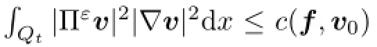
This point-wise approach is fundamentally unavailable in our case.The reason lies in two complications.First,we would obtain desired estimate only on a small time interval[0,Tdata], where Tdatadepends on c(f,v0)and we are not able to extend the solution on the whole time interval.Second,in short,we are not able to prove similar result to Lemma 3.51 in[17].

Let us relabel the interior cut-offunction by ξ0and the cut-offunctions localized near the boundary by ξk,k=1,2,···,N.Furthermore,we set θA(s)≡min(1+s,1+A).

where

ProofWe prove this statement in four steps following the main ideas from Lemma 4.15, [17].The frst three steps will show that we can get a similar(not identical)estimate on the time interval[0,T∗].The last step concludes the proof.

Step 1Second derivative estimates in the interior and in tangential directions near the boundary.

First we have

Using the estimate(1.7)we have

Moreover,using Young’s inequality,we obtain

Collecting the estimates together with those from[17]we obtain the interior estimate

The same procedure works for the estimate of the tangential derivatives.We obtain

Step 2Evaluation of all second derivatives of the velocity near the boundary in the terms of tangential derivatives.

We want to prove for q∈[1,2]the following estimate

Now,if we take the inequality(4.9)in the Lq-norm,take it to the r-th power and integrate over time,we get(4.8)provided that we can estimate the term containing G in a suitable way. For this purpose we proceed as in Section 3.5.3 using the curl-operator.

By Theorem 7.4 and the equations(3.29)and(3.30)we have for s=1,2

where the constant cnegis the constant from Theorem 7.4 and c is a generic constant which difers at each term.Notice the presence of time integration which is necessary in contrast to similar procedure in[17].Now,we easily deduce that

By similar steps

and with the help of the inequality(1.7),H¨older’s inequality and Young’s inequality for convolution we estimate

where we can use the fact that T∗is small enough and plug the last term into the left-hand side and get(4.8).

Step 3Inequalities for the full second velocity gradient.

Using this,the estimates(4.12)and(4.8),Remark 7.2 and Lemma 7.7 we compute

Putting the frst term on the right-hand side to the left yields the following inequality

which we wanted to prove.

Step 4Derivation of inequality(4.5).

From the estimate(4.13)it is easy to obtain the following inequality

where we also used the following estimate

valid for almost all t∈[0,T∗],which follows from the estimate(4.3)and the identity(3.17).

At last,we use the inequality(2.21)on the frst terms of the estimates(4.6)and(4.7). We add the result to the estimate(4.14)and obtain the inequality with the right-hand side bounded by the right-hand side of(4.14)(up to a multiplicative constant).

Therefore the proof is done. ?

ProofSee[17],Lemma 4.43.

4.2 Limiting Process

Lemma 4.4There exists a couple(vε,πε)such that for A→∞(or at least for a subsequences)

ProofSee[17](4.12).

Theorem 4.5The couple(vε,πε)from Lemma 4.4 satisfes the weak formulation of problem Pεon the time interval[0,T∗].

where∇(2)vεremain valid due to the weak lower semi-continuity of norms and(4.18).

Theorem 4.7The couple(vε,πε)is a strong solution of Problem Pεon[0,T∗].

but Lemma 4.3 together with the inequality(2.4)implies that also

Thus the proof is fnished.

4.3 Independence of the Estimates onA

We want to fnish this section with a few lemmas which are consequences of the estimate (4.5)if we pass to the limit as A→∞.We note that all these lemmas are originally from[17]. Thus for the detailed proof see the aforementioned paper.

Remark 4.10As a simple consequence we also get the inequality

5 Limit Passage for ε→0

5.1 Independence of the Estimates onε

At this point,we have for any ε＞0 a strong solution(vε,πε)of problem Pεon the time interval[0,T∗].However our estimates are still dependent on ε.First we recall notation

Moreover,we proved in Lemma 4.3,Lemma 4.9 and Remark 4.10 that

Lemma 5.1We denote

Then the estimate(5.6)implies that

ProofIt sufces to prove two inequalities.It immediately follows from Lemma 7.6 that

The second one follows from the inequality(2.3)

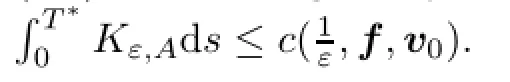
In the following,we estimate the right-hand sides of the estimates(5.2)-(5.7)uniformly with respect to ε.

Corollary 5.2The function vεis bounded in L∞(0,T∗;Vp)uniformly with respect to ε, i.e.,

Thanks to this inequality we can compute

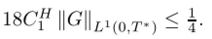
Finally,putting all of the above together with the estimate(5.4)brings us to the following inequality:

Using Gronwall’s lemma concludes the proof.

which together with the interpolation inequality

implies that

Therefore,we have the following estimate(immediately from(5.7),(5.9)and(5.11))

As a consequence,we obtain

which gives us the following estimate

Now,it sufces to use the inequality(5.8)to get the right hand sides of(5.4),(5.5)and (5.7)bounded independently of ε.

All together we just proved(using the inequality(??)from Lemma 7.7)that

5.2 Limiting Process

Lemma 5.3There exists a couple(v,π)such that for ε→0(or at least for a subsequence)

ProofThe proof is similar to those in previous sections.?

This means that the proof of Theorem 1.7 is fnished.

6 Extending the Solution on Time Interval[0,T]and Epilogue

At last,we have a strong solution(v,π)of Problem P on the time interval(0,T∗).We now present an informal comment why we cannot extend it on the whole time interval(0,T).

Time T∗fulfls the conditions(3.1),i.e.,it depends only on constants independent of f or v0,which is ideal.We would like to proceed as in[4]and thus,we defne

All together,we obtained a new result about regularity of weak solution for given problem. Furthermore,we provided explicit reasons why the regularity method used in[17]is not completely transferable for our model.There are two main reasons for this.First,the regularity estimates in Lemma 4.2 are unavailable due the point-wise nature of the method.Second,the need of strong regularity of the external body force f disables the extension of the solution to the whole time interval.

7 Appendix

7.1 Lebesgue and Sobolev Spaces

ProofIt follows immediately from the identity

Theorem 7.3([17],Lemma 6.5)Let Ω∈RNbe a domain,∂Ω∈C1and let u∈W1,2(Ω)N,ξ∈D(Ω).Then

7.2 Bochner Spaces

Theorem 7.5([10],Theorem 5.9.2)Let u∈W1,p(0,T;X)for some 1≤p≤∞,where X is a Banach space.Then u∈C([0,T];X)(after possibly being redefned on a set of measure zero).

7.3 General Auxiliary Results for Approximations

In this section we assume that the potential φFsatisfes assumptions(1.4)-(1.6)and φFAis given by Defnition 2.6.We denote Ip,q(u)≡RΩ(1+|D(u)|)q(p-2)|∇(Du)|qdx,where p≥2 and q≥1.

Lemma 7.6([17],Lemma 6.9)Let p≥2 and q∈[1,∞).Then there exist constants C17,C18,C19such that

Lemma 7.7([17],Lemma 6.12)Let p≥2 and q∈[1,∞)and let χAbe the characteristic function of the set{x∈Ω:|D(u(x))|≤A}.Then there exist constants C20,C21,C22such that

AcknowledgementsThe author would like to thank the scholarship of the Charles University center for mathematical modelling,applied analysis and computational mathematics (MathMAC).

[1]Agranovich Y Y,Sobolevskii P E.Motion of nonlinear viscoelastic fuid//Nonlinear Variational Problems and Partial Diferential Equations.Isola d’Elba,1990,1-12,Pitman Res Notes Math Ser,320.Harlow: Longman Sci Tech,1995

[2]Agranovich Y Y,Sobolevskii P E.Motion of nonlinear visco-elastic fuid.Nonlin Anal TMA,1998,32(6): 755-760

[3]Bae H-O,Wolf J.Existence of strong solutions to the equations of unsteady motion of shear thickening incompressible fuids.Nonlinear Anal Real World Appl,2015,23:160-182

[4]B´arta T.Global existence for an Oldroyd-type model for viscoelastic fuids.Riv Mat Univ Parma,2013, 4(1):37-54

[5]Bul´ıˇcek M,Ettwein F,Kaplick´y P,Praˇz´ak D.On uniqueness and time regularity of fows of power-law like Non-Newtonian fuids.Math Meth Appl Sci,2010,33(16):1995-2010

[6]Da Veiga H B,Kaplick´y P,R˚uˇziˇcka M.Boundary regularity of shear thickening fows.J Math Fluid Mech, 2011,13:387-404

[7]Diening L,R˚uˇziˇcka M,Wolf J.Existence of weak solutions for unsteady motions of generalized Newtonian fuids.Ann Sc Norm Super Pisa Cl Sci,2010,9(5)(1):1-46

[8]Dmitrienko V T,Zvyagin V G.On weak solutions of a regularized model of a viscoelastic fuid.(Russian) Difer Uravn,2002,38(12):1633-1645;translation in Difer Equ,2002,38(12):1731-1744

[9]Dmitrienko V T,Zvyagin V G.On strong solutions of an initial-boundary value problem for a regularized model of an incompressible viscoelastic medium.(Russian)Izv Vyssh Uchebn Zaved Mat,2004,9:24-40; translation in Russian Math(Iz VUZ),2005,48(9):21-37

[10]Evans L C.Partial Diferential Equations.Amer Math Soc,1998

[11]Gripenberg G,Londen S O,Stafans O J.Volterra Integral and Functional Equations.Cambridge:Cambridge Univ Press,1990

[12]Gyarmati I.Non-Equilibrium Thermodynamics.Field Theory and Variational Principles.Heidelberg: Springer,1970

[13]Ladyzhenskaya O A.On some new equations describing dynamics of incompressible fuids and on global solvability of boundary value problems to these equations.Trudy Steklov’s Math Institute,1967,102: 85-104

[14]Ladyzhenskaya O A.On some modifcations of Navier-Stokes equations for large gradients of velocity. Zapiski Nukhnych Seminarov LOMI,1968,7:126-154

[15]Ladyzhenskaya O A.The Mathematical Theory of Viscous Incompressible Flow.New York:Gordon and Breach,1969

[16]M´alek J,Neˇcas J,Rokyta M,R˚uˇziˇcka M.Weak and Measure-Valued Solutions to Evolutionary Partial Diferential Equations.Applied Mathematics and Mathematical Computation,Vol 13.Chapman and Hall, 1996

[17]M´alek J,Neˇcas J,R˚uˇziˇcka M.On weak solutions to a class of non-newtonian incompressible fuids in bounded three-dimensional domains:the case p≥2.Adv Difer Equ,2001,6(3):257-302

[18]Neˇcas J.Sur les normes quivalentes dans Wkp(Ω)et sur la coercivit des formes formellement positives//Sminaire Equations aux Drives Partielles,Montreal,1966

[19]Orlov V P,Sobolevskii P E.On mathematical models of a viscoelasticity with a memory.Diferential and Integral Equations,1991,4(1):103-115

[20]Pokorn´y M.Navier-Stokes Equations.Teaching script of MFF UK,http://www.karlin.mf.cuni.cz/～pokorny/NavierandStokes eng.pdf.

[21]Soukup I.Weak Solutions to the Class of Nonlinear Integrodiferential Equations[D].MFF UK,2012

[22]Vorotnikov D A,Zvyagin V G.On the convergence of solutions of a regularized problem for the equations of motion of a Jefery viscoelastic medium to the solutions of the original problem.(Russian)Fundam Prikl Mat,2005,11(4):49-63;translation in J Math Sci(NY),2007,144(5):4398-4408

[23]Wolf J.Existence of weak solutions to the equations of non-stationary motion of non-Newtonian fuids with shear rate dependent viscosity.J Math Fluid Mech,2007,9(1):104-138

∗Received August 7,2014;revised February 24,2015.This work was supported by Grant Agency of the Charles University(454213).