SPH and FEM Investigation of Hydrodynamic Impact Problems

Al-Bahkali Essam,Souli Mhamedand Al-Bahkali Thamar

1 Introduction

In the last decade in computational mechanics there is a growing interest in developing meshless methods and particle methods as alternatives to traditional FEM(Finite Element Method).Among the various meshfree and particle methods,Smoothed Particle Hydrodynamics(SPH)is the longest established and is approaching a mature stage.SPH is a Lagrangian meshless method in which the problem to be solved is discretized using particles that are free to move rather than element tied by connectivity mesh.SPH method has been extensively used for high impact velocity applications,in aerospace and defense industry for problems where classical FEM methods fail due to high meshes distortion.For small deformation,FEM Lagrangian formulation can solve structure interface and material boundary accurately,the main limitation of the formulation is high mesh distortion for large deformation and moving structure.One of the commonly used approach to solve these problems is the ALE(Arbitrary Lagrangian Eulerian)formulation which has been used with success for simulation of fluid structure interaction with large structure motion such as sloshing fuel tank in automotive industry and bird impact in aeronautic industry.It is well known from previous analysis,see Aquelet et al.(2005),that the classical FEM Lagrangian method is not suitable for most of the FSI problems due to high mesh distortion in the fluid domain.To overcome difficulties due to large mesh distortion,ALE formulation has been the only alternative to solve fluid structure interaction for engineering problems.For the last decade,SPH and DEM(Discrete Element Method),have been used usefully for engineering problems to simulate high velocity impact problems,high explosive detonation in soil,underwater explosion phenomena,and bird strike in aerospace industry,see Han et al.(2014)for details description of DEM method.SPH is a mesh free Lagrangian description of motion that can provide many advantages in fluid mechanics and also for modelling large deformation in solid mechanics.For some applications,including underwater explosion and hydrodynamic impact on deformable structures,engineers have switched from ALE to SPH method to reduce CPU time and save memory allocation.Unlike ALE method,and because of the absence of the mesh,SPH method suffers from a lack of consistency than can lead to poor accuracy,as described in Randles et al.(1996)and Vignjevic et al.(2006).

In this paper,devoted to ALE and SPH formulations for fluid structure interaction problems,the mathematical and numerical implementation of FEM and SPH formulations are described.From different simulations,it has been observed that for the SPH method to provide similar results as FEM Lagrangian formulations,the SPH meshing,or SPH spacing particles needs to be finer than the ALE mesh,see Messahel et al.(2013)for underwater explosion problem.To validate the statement on fluid structure interaction problems,we perform a simulation of a hydrodynamic impact problem.In the simulation,the particle spacing of SPH method needs to be at least two times finer than ALE mesh.A contact algorithm is performed at the fluid structure interface for both SPH and ALE formulations.

In Section 2, the governing equations of ALE formulation are described. In this section,we discuss mesh motion as well as advection algorithms used to solve mass,momentum and energy conservation in ALE formulation.Section 3 describes the SPH formulation,unlike FEM formulation which based of the Galerkin approach,SPH is a collocation method.The last section is devoted to numerical simulation of water impact on a deformable structure using both FEM and SPH methods.To get comparable results between FEM and SPH,the particle spacing of SPH method needs to be at least two times finer than FEM mesh

2 ALE formulation

A brief description of the FEM formulation used in this paper is presented,additional details can be provided in Benson(1992).To solve fluid structure interaction problems,a Lagrangian formulation is performed for the structure and an ALE formulation for the fluid material.In general ALE description,an arbitrary referential coordinate is introduced in addition to the Lagrangian and Eulerian coordinates.The material derivative with respect to the reference coordinate can be described in equation(1).Thus substituting the relationship between material time derivative and the reference configuration time derivative leads to the ALE equations,

whereXiis the Lagrangian coordinate,xithe Eulerian coordinate,wiis the relative velocity.Let denote byvthe velocity of the material and byuthe velocity of the mesh.In order to simplify the equations we introduce the relative velocityw=v−u.Thus the governing equations for the ALE formulation are given by the following conservation equations:

(i)Mass equation.

(ii)Momentum equation.

σijis the stress tensor defined byσ=−p+τ,whereτis the shear stress from the constitutive model,andpthe pressure.The volumetric compressive stresspis computed though an equation of state,and the shear stress from material constitutive law.

(iii)Energy equation.

Note that the Eulerian equations commonly used in fluid mechanics by the CFD community,are derived by assuming that the velocity of the reference configuration is zero,u=0,and that the relative velocity between the material and the reference configuration is therefore the material velocity,w=v.The term in the relative velocity in(3)and(4)is usually referred to as the advective term,and accounts for the transport of the material past the mesh.It is the additional term in the equations that makes solving the ALE equations much more difficult numerically than the Lagrangian equations,where the relative velocity is zero.

There are two ways to implement the ALE equations,and they correspond to the two approaches taken in implementing the Eulerian viewpoint in fluid mechanics.The first way solves the fully coupled equations for computational fluid mechanics;this approach used by different authors can handle only a single material in an element as described for example in Benson(1992).The alternative approach is referred to as an operator split in the literature,where the calculation,for each time step is divided into two phases.First a Lagrangian phase is performed,in which the mesh moves with the material,in this phase the changes in velocity and internal energy due to the internal and external forces are calculated.The equilibrium equations are:

In the Lagrangian phase,mass is automatically conserved,since no material flows across element boundaries.

In the second phase,the advection phase,transport of mass,energy and momentum across element boundaries are computed;this may be thought of as remapping the displaced mesh at the Lagrangian phase back to its original for Eulerian formulation or arbitrary location for ALE formulation using smoothing algorithms.From a discretization point of view of(5)and(6),one point integration is used for efficiency and to eliminate locking,Belytschko et al.(1989),zero energy modes are controlled with an hourglass viscosity.A shock viscosity,with linear and quadratic terms developed by Von-Neumann and Richtmeyer(1950)is used to resolve the shock wave.The resolution is advanced in time with the central difference method,which provides a second order accuracy for time integration.

For each node,the velocity and displacement are updated as follows:

whereFintis the internal vector force andFextthe external vector force associated with body forces,coupling forces,and pressure boundary conditions,Mis a diagonal lumped mass matrix.For each element of the mesh,the internal force is computed as follows:

Bis the gradient matrix andNelemthe number of elements.

The time step size,Δt,is limited by the Courant stability condition[4],which may be expressed as:

wherelis the characteristic length of the element,andcthe sound speed of the element material.For a solid material,the speed of sound is defined as:

whereρis the material density,Kis the module of compressibility.

2.1 Moving mesh algorithm

The ALE algorithm used in the paper allows the fluid nodes to move in order to maintain the integrity of the mesh.As the fluid impacts the plate,the fluid mesh moves with a mesh velocity that is different from fluid particle velocity.The choice of the mesh velocity constitutes one of the major problems with the ALE description.Differen techniques have been developed for updating the fluid mesh domain.For problems defined in simple domains,the mesh velocity can be deduced through a uniform or non uniform distribution of the nodes along straight lines ending at the moving boundaries.This technique has been used for different applications including water wave problems.For general computational domains,the mesh velocity is computed through partial differential equations,with appropriate boundary conditions.

This technique has been used by different authors,where the mesh is modeled as a linear or nonlinear elastic material(10)-(12),and can be computed through partial differential equation with appropriate boundary conditions:

where σmeshis the stress tensor for mesh motion,given by

ε is the deformation tensor,the mesh displacement at node i,and C the constitutive matrix.C can be element dependant such that smaller element can undergo lesser deformation.The constitutive matrix coefficients are inversely proportional to element size.

For some CFD and general FSI problems,authors consider the mesh as a viscous fluid material.This process can be described by a classical diffusion equation for mesh velocity associated with appropriate boundary conditions:

µmeshdesignates mesh viscosity that can be space dependant.

For some three dimensional dynamic problems,solving elasticity equations(10)-(12)or(13)for mesh motion can be insuf fi cient and after some time steps node displacement leads to high mesh distortion and negative element Jacobian before termination time.To prevent high mesh distortion,a combination of elasticity model with simple average algorithm is used in the paper.Simple averaging of the displacement of the surrounding nodes allows the mesh to be more uniform,since this algorithm is nonlinear;few iterations are processed to smooth the mesh.

where N in equation(14)is the number of surrounding nodes.Equation(14)is combined with equation(10)-(12),with a smaller scale factor for the simple average equation This combination has been successfully used for a broad range of problems,including impact problems,and underwater explosion problems using a single material ALE formulation.One of the inconveniences of using simple average is that it tends to eliminate the mesh grading in the material domain,and tendsto smooth out any steep gradient between elements.The new displacement of node is given by(15).

For normalization purposeα1andα2are positive coefficients satisfying equation(16)

2.2 Advection phase

In the second phase,the transport ofmass,momentum and internal energy across the element boundaries is computed.This phase may be considered as a‘remapping’phase.The displaced mesh from the Lagrangian phase is remapped into the initial mesh for an Eulerian formulation.To illustrate the advection phase,we consider in figure 1,a simple problem with 2 different materials,one with high pressure and the second a lower pressure.During the Lagrangian phase,material with high pressure expands,and the mesh moves with the material.Since we are using Eulerian formulation,the mesh is mapped to its initial configuration,in the advection phase,material volume called flux is moving from element to element,but we keep separate materials in the same element,using interface tracking between materials inside an element

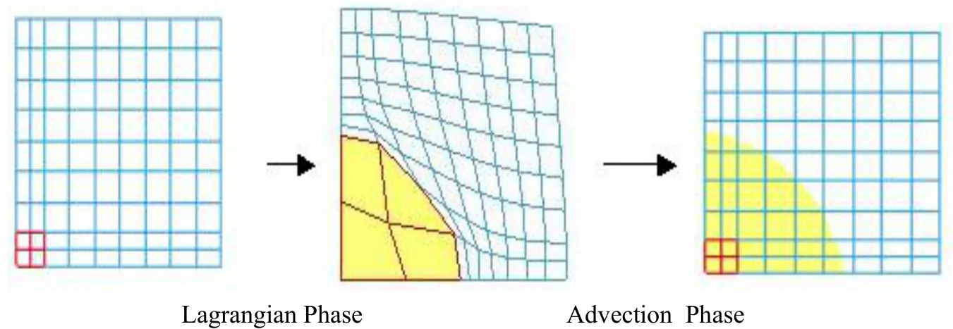
Figure 1: Lagrangian and Advection Description.

Conservation properties are performed during the Lagrangian phase;stress computation,boundary conditions,contact forces are computed.The advection phase can be seen as a remapping phase from a deformable mesh to initial mesh for an Eulerian formulation,or to an arbitrary mesh for general ALE formulation.In the advection phase,volume flux of material through element boundary needs to be computed.

Once the flux on element faces of the mesh is computed,all state variables are updated according to the following algorithm,using a finite volume algorithm(17),

where the superscripts‘-’and‘+’refer to the solution values before and after the transport.Values that are subscripted by j refer to the boundaries faces of the element,through which the material flows,and theFluxjare the volume fluxes transported through adjacent elements.The flux is positive if the element receives material and negative if the element looses material.

The ALE multi-material method is attractive for solving a broad range of non-linear problems in fluid and solid mechanics,because it allows arbitrary large deformations and enables free surfaces to evolve.The advection phase of the method can be easily implemented in an explicit Lagrangian finite element code.

3 SPH Formulation

The SPH method developed originally for solving astrophysics problem has been extended to solid mechanics by Libersky et al.(1993)to model problems involving large deformation including high impact velocity.SPH method provides many advantages in modeling severe deformation as compared to classical FEM formulation which suffers from high mesh distortion.The method was first introduced by Lucy(1977)and(2010)and Monaghan et al.(1983),for gas dynamic problems and for problems where the main concern is a set of discrete physical particles than the continuum media.The method was extended to solve high impact velocity in solid mechanics,CFD applications governed by Navier-Stokes equations,and fluid structure interaction problems.It is well known from previous papers,Vila(1999)that SPH method suffers from lack of consistency that can lead to poor accuracy of motion approximation.

A detailed overview of the SPH method is developed by Liu et al(2010),where the two steps for representing a continuous function,using integral interpolation and kernel approximation are given by(18)and(19),

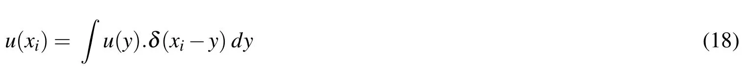
where the Dirac function satis fi es:

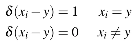
Figure 2: Particle spacing and Kernel function.

The approximation of the integral function(18)is based on the kernel approximation W,that approximates the Dirac function based on the smoothing length h,figure 2,

that represents support of the kernel function.SPH interpolation is given by the following equation(19):

Unlike FEM,where weak form Galerkin method with integration over mesh volume,is common practice to obtain discrete set of equations,in SPH since there is no mesh,collocation based method is used.In collocation method the discrete equations are obtained by enforcing equilibrium equations,mass,linear momentum and energy,at each particle.In SPH method,the following equations are solved for each particle(20),

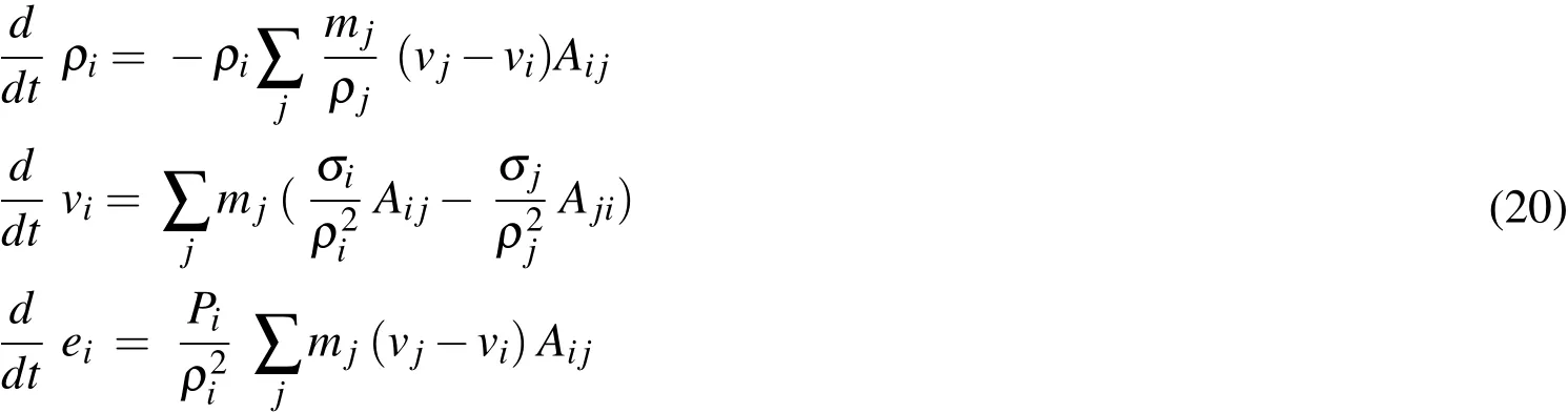
whereρi,vi,eiare density,velocity and internal energy of particle,σi,miare Cauchy stress and particle mass.

Aijis the gradient of the kernel function defined by(21)

It had be shown that convergence and stability of the SPH methods depends on the distribution of particles in the domain,

4 Constitutive material models for water and plate

4.1 Constitutive material model for water

In this paper a Newtonian fluid constitutive material law is used water,see table 1.For pressure response,Mie Gruneisen equation of state is used with parameters defined in table 2,which defines material’s volumetric strength and pressure to density ratio.Pressure in Mie Gruneisen equation of state is defined by equation(22)

Where c is the bulk speed of sound,whereρ0andρare the initial and current densities.The coefficient s is the linear Hugoniot slope coefficient of the shock velocity particle velocity(Us−Up)curve,equation(23),

Usis the shock wave velocity,Upis the particle velocity.This equation of state requires fluid speci fi c coefficient s,which is obtained through shock experiment by curve fi tting of theUs−Uprelationship.Shock experiments on fluids and solids provide a relation between the shock speedUsand the particle velocity behind the shock,Upalong the locus of shocked states.

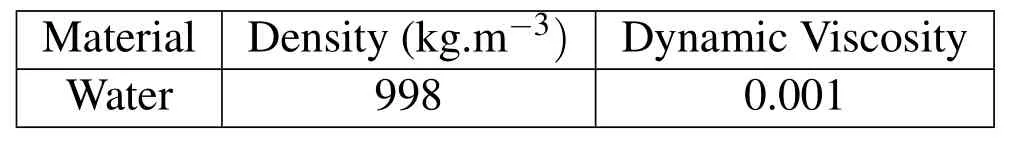
Table 1: Material data for water.

An important phenomenon that arises during hydrodynamic impact is the formation of shock,mathematically equations(18)-(20)develop a shock,which lead tonon continuous solution and the problem is well posed only if the shock conditions are satisfied.These conditions called Rankine Hugoniot conditions describe the relationship between the states on both sides of the shock for conservation of mass,momentum and energy across the shock,and are derived by enforcing the conservation laws in integral form over a control volume that includes the shock In the absence of numerical viscosity,high non physical oscillations are generated in the immediate vicinity of the shock..

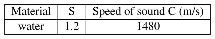
Table 2: Mie-Gruneisen Equation of state.

4.2 Constitutive material models for the plate

For the structure,an elastic plastic with isotropic hardening constitutive material law is used.In isotropic hardening,the center of the yield surface is fixed but the radius is a function of the plastic strain,this material is described in detail in Hallquist(1998).Material properties for the plate are given in the table 3

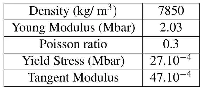
Table 3: Parameters used for Structure.

The plate is modeled with using 4-noded Belyschko-Lin-Tsay type shell elements Belyschko et al.(2000),with fi ve integration points through the thickness,in order to accurately describe the fl exion of the plate.Belyschko-Lin-Tsay shell element is based on a combined co-rotational and velocity-strain formulation.The efficiency of the element is obtained from mathematical simplifications that result from these two kinematical assumptions.Because of its computational efficiency,this formulation becomes the shell element formulation for explicit time integration calculations

5 Numerical Simulations

5.1 SPH formulation

De fi nition of proper boundary conditions for SPH formulation is a challenge in the SPH theory.Several techniques have been developed in order to enhance the desired condition,to stop particle from penetrating solid boundaries and also to complete the truncated kernel by the physical domain.Among the different techniques,the ghost particle method known to be robust and accurate,has been implemented in LS-DYNA,and used in this simulation,Hallquit(1998).When a particle is close to the boundary,it is symmetrised across the boundary with the same density,pressure as its real particle such that mathematical consistency is restored.For most simulations,host particles velocity is adjusted so that slips or stick boundary condition is applied.

In order to treat problem involving discontinuities in the fl ow variables such as shock waves an additional dissipative term is added as an additional pressure term.This artificial viscosity should be acting in the shock layer and neglected outside the shock layer.In this simulation a pseudo-artificial pressure termµijderived by Monoghan et al.(1983)is used.This term is based on the classical Von Neumann artificial viscosity and is readapted to the SPH formulation as follow,

5.2 Fluid-Structure Contact Algorithm

For SPH and ALE simulations,a penalty type contact is used to model the interaction between the fluid and the plate.In computational mechanics,contact algorithms have been extensively studied by several authors.Details on contact algorithms can be found in Belyshko et al.(1989).Classical implicit and explicit coupling are described in detail in Longatte et al.(2003),where hydrodynamic forces from the fluid solver are passed to the structure solver for stress and displacement computation.In this paper,a coupling method based on penalty contact algorithm is used.In penalty based contact,a contact force is computed proportional to the penetration depth,the amount the constraint is violated,and a numerical stiffness value.In an explicit FEM method,contact algorithms compute interface forcesdue to impact of the structure on the fluid,these forces are applied to the fluid and structure nodes in contact in order to prevent a node from passing through contact interface.In contact one surface is designated as a slave surface,and the second as a master surface.The nodes lying on both surfaces are also called slave and master nodes respectively.The penalty method imposes a resisting force to the slave node,proportional to its penetration through the master segment,as shown in figure 3 describing the contact process.This force is applied to both slave and nodes of the master segment in opposite directions to satisfy equilibrium.Penalty coupling behaves like a spring system and penalty forces are calculated proportionally to the penetration depth and spring stiffness.The head of the spring is attached to the structure or slave node and the tail of the spring is attached to the master node within a fluid element that is intercepted by the structure,as illustrated in figure 3.Similarly to penalty contact algorithm,the coupling force is described by(25):

wherekrepresents the spring stiffness,anddthe penetration.The forceFin figure 3 is applied to both master and slave nodes in opposite directions to satisfy force equilibrium at the interface coupling,and thus the coupling is consistent with the fluid-structure interface conditions namely the action-reaction principle.

The main difficulty in the coupling problem comes from the evaluation of the stiffness coefficientkin Eq.(25).The stiffness value is problem dependent,a good value for the stiffness should reduce energy interface in order to satisfy total energy conservation,and prevent fluid leakage through the structure.The value of the stiffnesskis still a research topic for explicit contact-impact algorithms in structural mechanics.In this paper,the stiffness value is similar to the one used in Lagrangian explicit contact algorithms.The value ofkis given in term of the bulk modulusKof the fluid element in the coupling containing the slave structure node,the volumeVof the fluid element that contains the master fluid node,and the average areaAof the structure element connected to the structure node.

5.3 ALE Mesh sensitivity analysis for SPH Method

A detailed finite element model was developed to represent a hydrodynamic impact problem.Before conducting the simulation,mesh sensitivity tests were performed for the finite element model on a rigid plate for which analytical solution is available in the literature.The fluid domain consists of a cube with a side of length 10 cm,impacting the plate with impact velocity of 100m/s.Three different mesh densities were used for mesh sensitivity tests from 900 to 7000 hexahedra elements for the fluid mesh.Simulation of the three finite element meshes gives same results with good correlation with analytical solution for impact on a rigid plate.Theoptimal model of 900 elements was taken as reference solution for the finite element simulation.The structure under consideration is a square plate.The dimensions of the plate,which is presented in figure 4,are 0.3 m by 0.3 m with a thickness of 1 mm The plate is constrained at the two edges in translation and rotation,details of the problem description is shown if figure 4.For the SPH simulations,two different models have been used,the first model has a number of particles similar to the number of nodes in the FEM model,which consists of 1440 particles,the second model consists of 27000 particles with same mass.

Figure 3: Contact algorithm description.

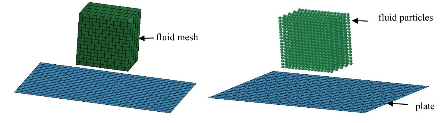
Figure 4: FEM and ALE description.

For the ALE simulation smoothing algorithm described in previous section is performed on the fluid mesh,to prevent high mesh distortion,as shown in figure 5.

Hydrodynamic contact forces on the plate for both ALE and SPH methods are computed and compared.Large discrepancy between the two results can be observed in terms of hydrodynamic resultant impact force on the plate as shown in figure 7.Momentum impulse can be deduce by integrating over time the resultant impact force,and both results are different as it can be observed in figure 8.We alsohave observed discrepancy between SPH and FEM models for displacement and velocity of the plate center as shown in figure 9 and 10.

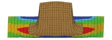
Figure 5: Fluid mesh smoothing during impact.

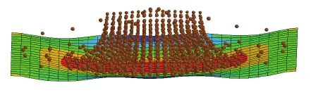
Figure 6: Coarse SPH model during impact.

To improve SPH results and to obtain good correlation with ALE model, finer particle spacing needs to be performed for SPH simulation.SPH re fi nement can be performed by decreasing particle pacing by a factor of two which can be achieved by increasing the number of SPH particles from 1440 to 7000 as shown in figure 11,to clarify both SPH discretizations we show the two SPH models in figure 12.By re fi ning the SPH model we achieved good correlations between SPH and ALE models in term of resultant force,momentum impulse on the plate figure 13 and figure 14,as well as displacement and velocity at the center of the plate figure 15 and figure 16.The price that need to be paid for efficiency of SPH method,is that the SPH method may need larger number of particles to achieve an accuracy comparable with that of a mesh based method.

As mentioned in the introduction,experimental tests for hydrodynamic on an elasto-structures,are costly to perform.In order to validate the SPH technique described in the paper,the ALE formulation can be used for validation,since ALE solution is accurate for times where the mesh is deformed but not highly distorted.

The biggest advantage the SPH method has over ALE methods is that it avoids the

heavy tasks of re-meshing.For some complex fluid structure interaction simulations where elements need to be eroded due to failure,the ALE remeshing method fails,since a new element connectivity needs to be regenerated.SPH method allows failure particles by deactivating failed particles for the particle loop processing.This is a major advantage that SPH method has over classical ALE methods.To further improve the accuracy of the SPH method for the simulation of free surface and impact problems,efficiency and usefulness of the two methods,often used in numerical simulations,are compared.

Figure 7: Time history of Resultant force(N)on the plate with ALE and coarse SPH.

Figure 8: Time history of Resultant impulse(N.sec)on the plate with ALE and coarse SPH.

Figure 9: Time history of vertical velocity at the center plate with FEM and coarse SPH.

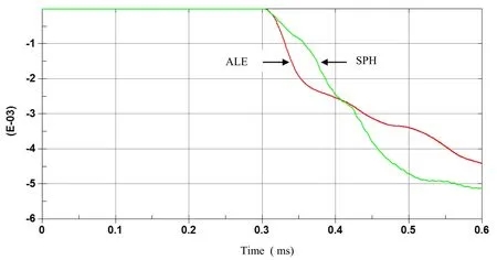
Figure 10: Time history of vertical displ(m)at the center plate on the plate with ALE and coarse SPHH.

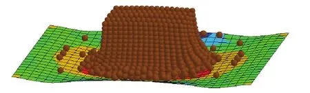
Figure 11: Finer SPH simulation during impact.

Figure 12: Coarse and fi ne SPH simulations during impact.

Figure 13: Time history of Resultant force(N)on the plate with ALE and finer SPH.

Figure 14: Time history of Resultant Impulse(N.sec)on the plate with ALE and finer SPH.

Figure 15: Time history of vertical velocity(m/s)at the center plate with ALE and finer SPH.

Figure 16: Time history of vertical displ(m)at the center plate with ALE and finer SPH.

6 Conclusion

For structure integrity and safety,several efforts have been made in defense and civilian industries,for modeling hydrodynamic impacts and their effect on structures.In aerospace industry,engineers move from mesh based method to SPH method to simulate bird impact on deformable structure.We also observed in defense industry where SPH method is recently used for undermine explosion problem and their impact on the surrounding structure.

The biggest advantage the SPH method has over mesh based mesh methods is that it avoids the heavy tasks of re-meshing for hydrodynamic problems or structural problems with large deformation.The price to be paid for efficiency is that the SPH method may need finer resolution to achieve accuracy comparable with that of a mesh based.As a result,SPH simulation can be utilised by using finer particle spacing for applications where mesh based method cannot be used because of remeshing problems due to high mesh distortions.Since the ultimate objective is the design of a safer structure,numerical simulations can be included in shape design optimization with shape optimal design techniques(see Barras et al(2012)),and material optimization(see Gabrys et al(2012)).Once simulations are validated by test results,it can be used as design tool for the improvement of the system structure involved.

Acknowledgement:The authors are grateful to the College of Engineering Research Center at King Saud University,for the support of this work.

Aquelet,N.;Souli,M.;Olovson,L.(2005):Euler Lagrange coupling with damping effects:Application to slamming problems.Computer Methods in Applied Mechanics and Engineering,vol.195,pp.110-132.

Barras,G.;Souli,M.;Aquelet,N.;Couty,N.(2012):Numerical simulation of underwater explosions using ALE method.The pulsating bubble phenomena.Ocean Engineering,vol.41,pp.53-66.

Belytschko,T.;Liu,W.K.;B.Moran.(2000):Nonlinear Finite Elements for Continua and Structure.Wiley&sons.

Benson,D.J.(1992):Computational Methods in Lagrangian and Eulerian Hydrocodes.Computer Methods in Applied Mechanics and Engineering,vol.99,pp.235-394.

Colagrossi,A.;Landrini,M.(2003):Numerical simulation of interfacial flows by smoothed particle hydrodynamics.Journal of Computational Physics,vol.191,pp.448.

Gingold,R.A.;Monaghan,J.J.(1977):Smoothed particle hydrodynamics:theory and applications to non-spherical stars.Monthly Notices of the Royal Astronomical Society,vol.181,pp.375–389.

Hallquist,J.O.(1998):LS-DYNA Theory Manuel.Livermore Software Technology Corporation,California USA.

Han,Z.D.;Atluri,S.N.(2014):On the Meshless Local Petrov-Galerkin MLPGEshelby Methods in Computational Finite Deformation Solid Mechanics-Part II.CMES:Computer Modelling in Engineering&Sciences,vol.97,no.3,pp.199-237.

Libersky,L.D.;Petschek,A.G.;Carney,T.C.;Hipp,J.R.;Allahdadi,F.A.(1993):High Strain Lagrangian Hydrodynamics:A Three-Dimensional SPH CODE for Dynamic Material Response.Journal of Computational Physics,vol.109,pp.67-75.

Liu,M.B.;Liu,G.R.(2010):Smoothed Particle Hydrodynamics(SPH):an Overview and Recent Developments.Archives of Computational Methods in Engineering,vol.17,pp.25–76.

Longatte,L.;Bendjeddou,Z.;Souli,M.(2003):Application of Arbitrary Lagrange Euler Formulations to Flow-Inuced Vibration problems.Journal of Pressure Vessel and Technology,vol.125,pp.411-417.

Lucy,L.B.(1977):A numerical approach to the testing of fi ssion hypothesis.The Astronomical Journal,vol.82,pp.1013–1024.

Messahel,R.;Souli,M.(2013):SPH and ALE Formulations for Fluid Structure Coupling.CMES:Computer Modeling in Engineering&Sciences,vol.96,no.6,pp.435-455.

Monaghan,J.J.;Gingold,R.A.(1983):Shock Simulation by particle method SPH.Journal of Computational Physics,vol.52,pp.374-389.

Ozdemir,Z.;Souli,M.;Fahjan Y.M.(2010):Application of nonlinear fluid–structure interaction methods to seismic analysis of anchored and unanchoredtanks.Engineering Structures,vol.32,pp.409-423.

Randles,P.W.;Libersky,L.D.(1996):Smoothed Particle Hydrodynamics:Some recent improvements and applications.Computer Methods in Applied Mechanics and Engineering,vol.139,pp.375-408.

Souli,M.;Gabrys,J.(2012):Fluid Structure Interaction for Bird Impact Problem:Experimental and Numerical Investigation.CMES:Computer Modeling in Engineering&Sciences,vol.2137,no.1,pp.1-16.

Vignjevic,R.;Reveles,J.;Campbell,J.(2006):SPH in a Total Lagrangian Formalism.CMES:Computer Modelling in Engineering and Science,vol.14,pp.181-198.

Vila,J.(1999):On particle weighted method and smoothed particle hydrodynamics.Mathematical Models and Method in Applied Science,vol.9,pp.161-209.