
Production Line Capacity Planning Concerning Uncertain Demands for a Class of Manufacturing Systems with Multiple Products
2015-08-09 02:01HaoLiuQianchuanZhaoNingjianHuangandXiangZhao
Hao Liu,Qianchuan Zhao,Ningjian Huang,and Xiang Zhao
Production Line Capacity Planning Concerning Uncertain Demands for a Class of Manufacturing Systems with Multiple Products
Hao Liu,Qianchuan Zhao,Ningjian Huang,and Xiang Zhao
—In this paper,we study a class of manufacturing systems which consist of multiple plants and each of the plants has capability of producing multiple distinct products.The production lines of a certain plant may switch between producing different kinds of products in a time-sharing mode.We optimize the capacity con fi guration of such a system′s production lines with the objective to maximize the overall pro fi t in the capacity planning horizon.Uncertain demand is incorporated in the model to achieve a robust con fi guration solution.The optimization problem is formulated as a nonlinear polynomial stochastic programming problem,which is dif fi cult to be ef fi ciently solved due to demand uncertainties and large search space.We show the NP-hardness of the problem fi rst,and then apply ordinal optimization(OO)method to search for good enough designs with high probability.At lower level,an mixed integer programming (MIP)solving tool is employed to evaluate the performance of a design under given demand pro fi le.
Index Terms—Capacity planning,uncertain demands,ordinal optimization(OO).
I.INTRODUCTION
MASS customization has been recognized as one of the new paradigms for today′s automotive manufacturing. As auto companies increase their manufacturing fl exibility,a vehicle assembly plant usually possesses capability of producing multiple distinct vehicle models in order to meet rapidly changing market and gain competitive advantages.As a result of such a paradigm change,automotive companies having a global manufacturing network need urgently a planning tool that helps to allocate production/assembly lines into multiple plants and to fi nd an optimal solution of line capacity con fi guration to meet the uncertain market demands.Such decisions are believed to in fl uence the performance of a manufacturing network and thus the company′s competitiveness[1].
Motivated by practical backgrounds,this paper is exploring ways to meet these challenges.We studied a class of manufacturing systems,of which the features will be described and modeled in detail in Section II.We tried to address the problem of optimizing the capacity con fi guration of the production lines in the system,with the objective to maximize the overall pro fi t in the capacity planning horizon(often several years). Incorporating the future uncertain demand,the problem is formulated into a two-stage stochastic nonlinear programming problem with the fi rst stage comprising capacity con fi guration decisions and the second stage with production decisions. The solution of the capacity con fi guration will eventually determine the company′s investment on its production lines.
The class of manufacturing systems studied in this paper is modeled mainly based on our practical investigation.In current literature,limited study is found that investigates a manufacturing system like the class we study here.Similar studies on planning production lines′capacity for manufacturing systems exist in literature but such studies focus on various systems featuring in different characteristics.The most similar study,for example,is planning strategic multisite and multi-product production networks.Reference[1]reported the BMW′s global production network and its planning with investment,production and supply chain optimization incorporated.Reference[2]planned the strategic network for an international automotive manufacturer,focusing on the decisions of allocating products to different plants and expanding the capacity of a given manufacturing network with fi xed plant locations.Reference[3]also modeled and optimized the production planning in the automotive industry under uncertain demands,including tactical aspects such as workforce planning.References[4]and[5]are other two recent examples.However,the system studied in this paper has some features that are not considered in the above literature, and thus is differently modeled and solved.The features are described at the beginning of Section II.
For two-stage stochastic programming,techniques such as Bender′s decomposition(as in[3]and[6])or tools such as Lingo(as in[7])could be applied.Although these are relatively ef fi cient ways and are possible to be further accelerated,the computation burden would still be too large to handle within limited time if the problem is of a large scale or if the solution performance estimation is time-consuming. To address this,a solution framework will be proposed in this paper applying ordinal optimization(OO)[8]to fi nd good enough solutions with high probability.The details of the framework will be given in Section III-C.
The rest of the paper is organized as follows.In Section II,we will introduce the related concepts of the manufacturing system we investigated and then give a general formulation of the problem.In Section III,we will analyze the problem and fi nd ways to solve it.In Section IV,numerical results will be presented.Section V concludes the paper.
II.THEPLANNINGPROBLEM:A GENERALMODEL
We propose in this section a general model of the production line capacity planning problem of a class of manufacturing system.The class of manufacturing system we considered here has a basic feature that the system consists of multiple plants(usually located at different places geographically)and each of the plants has capability of producing multiple distinct products.Some of the products and their production processes are similar,and their production processes are similar,and the production lines could switch between producing any kind of them only with minor modi fi cations of the equipment,tooling or the equipment con fi gurations.However,the modi fi cations are not dramatic to produce totally different products.Fig.1 gives a schematic example of such a manufacturing system.In the example,products A and B are similar,but product C is not.Plants 1 and 2 have production lines capable of producing both products A and B.Plant 1 also has production lines capable of producing product C.Plant 3 only has production lines capable of producing product C.
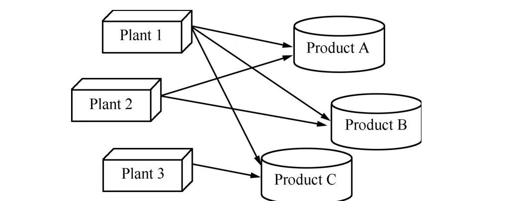
Fig.1.Schematic example of the class of manufacturing system considered in this paper.
A typical example of such a manufacturing system is one that consists of several vehicle assembly plants of an auto manufacturing company.Those assembly plants may be located at different places and could individually produce different models of vehicles.A production line of a vehicle assembly plant usually consists of two parallel sub-lines–vehicle assembly sub-line makes the body;powertrain assembly sub-line makes the chassis;the body and chassis are fi nally assembled together to produce a vehicle.The lines can be shared by the assembly of different vehicle models.A plant could choose to produce some models of vehicles according to its geographical characteristics,product strategies,and forecasted global or regional market demands for speci fi c vehicle models,etc.
A.Related Concepts of the Manufacturing System
Uncertainty
When addressing the production line capacity planning problem for a manufacturing system,we face many respects of uncertainty such as the market demand,states of the machines(working or failure),raw material prices and product prices.In this paper,we only consider the uncertainty of the market demand,since this is always the most fundamental and challenging uncertainty at a planning stage.In the planning stage,we can always assume plants have similar reliability in a statistical manner.By this assumption the modeling could be simpli fi ed but without sacri fi cing the essential insights one could gain from planning.
Market demand forecasting is necessary for production capacity planning.This could be done by fi rst analyzing the historical sale data to gain some knowledge about the demand trends or distribution,and then forecasting based on the knowledge.Proper statistical techniques could be used for both analyzing and forecasting.Although the knowledge gained is important as a guide to forecast the future demand and facilitate reasonable planning,the demand in the past is hardly repeated in the future due to the inevitable uncertainty existing in the market.Therefore we have to take into account the randomness in addition to the basic knowledge to make the planning more robust.
Production rates of a plant
The production rate of a production line is de fi ned as the number of products produced by the line in per unit time. Here,we do not focus on any individual production line but a whole plant.When we talk about the line production rate of a plant,we see the production lines of the plant as a whole and consider their overall production rate,i.e.,the capacity of a plant is the sum of production rates of all products in this plant.
As mentioned before,the production lines of a plant may be used to produce different products.When considered as a whole,the production lines may have different production rate respectively for different products.There are mainly two reasons.One is that the process requirements of different products are different.The other is that the product-speci fi c equipment installed for different products varies.When the process requirement of a certain product is fi xed,the plant has to install more product-speci fi c equipment if there is a requirement from the plant to increase the production rate of a speci fi c product.
The amount of product-speci fi c equipment installed for different products in a plant in fact determine the plant′s respective maximum production rates for the products.Actually,this is what we need to decide before the production starts.In the optimization problem proposed in Section III,the maximum production rates are modeled as the key decision variables.
For a certain product,some equipment may not be running when the forecasted product demand is low.Thus,the respective actual production rates for different products may vary from time to time according to the production plan.
Production period
In our model,we use week as a unit time period.The period is de fi ned for the convenience of demand forecasting and production rate adjustment.First,we assume the demand forecasting gives the demand of different products for every week of the planning horizon.Second,we assume the plants could adjust their actual production rates for the products according to the forecasted demand at the beginning of every week and maintain the rates unchanged for the whole week.
Shift pattern,normal working time and overtime
The shift pattern adopted by a plant in a production period (week in our model)determines the plant′s total working time available in that period.A plant can adopt different shift patterns in different periods to achieve different levelsof total working time.The total working time includes two parts:normal working time and overtime.For instance,the workers could be divided into three crews,and are arranged for work in 3 shifts per day,each crew works in a shift for 8 hours.Each worker works normally for 5 days per week. Then the total normal working time in a week is 8 hrs/shift×3 shifts/day×5 days=120hrs.If the plant is needed to produce more in some week,an overtime day could be arranged.In this case,the overtime hours is 8hrs/shift×3 shifts/day×1 days=24hrs and the total working time available in the week is 120hrs+24hrs=144hrs.The overtime is an important fl exibility that a plant could utilize to achieve a high production volume when needed.
In our model,we assume for simplicity that the plants respectively adopt a fi xed shift pattern.Therefore,the total working time of the plants and the normal working time and overtime in each period are all deterministic.
Line sharing production
For a plant that could produce more than one kind of products,the production of the products will share the production lines of the plant.In our model,we assume the time allotment is discrete,for example,in unit of hours.
Plant capacity.The capacity of a plant in a period could be de fi ned by combining the plant′s line production rates for different products and its total working time available.For example,if a plant could produce product A and product B with respective production rates 60products/hr and 40 products/hr,and its total working time in a week is 120hrs, and then the plant′s weekly capacity is 60×120=7200 product A or 40×120=4800 product B,the same could be represented by Fig.2.

Fig.2.Schematic diagram of plant capacity.
Since the time allotment occurs when actual production starts,the capacity planning is con fi ned to the decision on maximum production rates con fi guration.
Cost pro fi le
We consider three aspects of costs in our model:
1)Investment cost:the cost of investment on production lines.The investment cost on the production line equipment for a product in a plant is a piecewise linear function of the corresponding maximum production rate of the product in the plant(Fig.3).
2)Set-up cost:the cost of setting up the equipment for production,including the cost of facilities installing,tooling exchange,line maintenance,etc.The set-up cost of producing a product in a plant in a period is positively correlated to the actual production rate of the product in the plant in that period. In our model,we assume the set-up cost is proportional to the actual production rate.

Fig.3.The relationship of investment cost and the maximum production rate.Note here a left-continuous function is adopted just for illustration.Our method also works for right-continuous cost functions.
3)Production cost,which includes two parts:
a)Consumption cost.the cost of material and energy consumption,wear and tear of facility and equipment,etc., which is proportional to the production.
b)Labor cost.the cost of labor.The labor cost is also proportional to the production but the proportionality coef fi cients are different for the production in normal working time and in overtime.Usually the former is lower than the later due to the extra payment to workers who are working overtime(Fig.4).
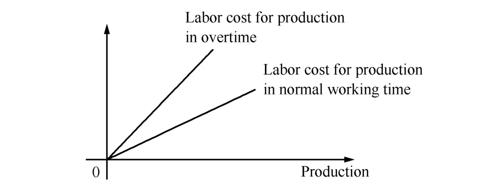
Fig.4.The relationship of labor cost and production.
Overproduction and underproduction
We assume in our model no inventory and thus no overproduction.However,underproduction is allowed but will cause a penalty.As we consider the underproduction happening more seriously in the near term than that in the future,a discount factor of penalty is introduced.
B.Problem Formulation
Our model aims at fi nding a proper design of the maximum production rates of different products for the plants at the beginning of a planning horizon.After the design is decided, the actual production in the plants cannot exceed the plants’respective maximum production rates.However,as mentioned above,the plants can adjust their actual production rates and the time allotment for different products periodically according to the forecasted demand.Thus,there are two stages of decisions in our problem.The fi rst stage decision is to decide the maximum production rates.The second stage decision, which is to be made relying on the fi rst stage decision,is to decide the actual production plan.
Considering the demand uncertainty,the capacity planning problem is formulated as a stochastic programming problem as follows.
Given values
i∈I:index of a plant.I={1,2,···,number of plants}.
j∈J:index of a product.J={1,2,···,number of products}.
t∈T:index of a period.T={1,2,···,number of periods}.
(,respectively):available normal working hours(overtime hours,respectively)of plantiin periodt. HIW stands for“hours In a week”,as we consider periods as weeks.
ICij(·):investment cost of the production equipment of productjin planti,which is a stepwise function ofJPHij0(to be introduced later).
scijt:set-up cost coef fi cient of setting up the production equipment for productjin plantiin periodt,which multiplied byJPHijt(to be introduced later)makes the set-up cost.If the productjis not being produced at plantiin periodt,thenscijtequals to 0.
ccijt:consumption cost per productjproduced in plantiin periodt.
(,respectively):labor cost per productjproduced in plantiin periodtin normal working hours(overtime hours, respectively).
pj:coef fi cient of penalty for underproduction of productj.
α:discount factor of penalty for underproduction.
wjt:selling price per productjin periodt.
djt:demand for productjin periodt(random variable). The vector of the demands will be denoted byddd.
Decision variables
First stage decision variables:
JPHij0:maximum production rate of productjin planti.JPH stands for“job per hour”.If plantidoes not produce productj,thenJPHij0=0.
The vector of the fi rst stage decision variables will be denoted by.A solution ofwill also be called a“design”hereinafter.
Second stage decision variables:
JPHijt:actual production line rate of productjin plantiin periodt.
(,respectively):normal working hours(overtime hours,respectively)allotted to productjin plantiin periodt.
The vector of the second stage decision variables will be denoted byxxx.
Objective function
For clarity,we write the following expressions before giving the objective function and constraints:
Investment cost:

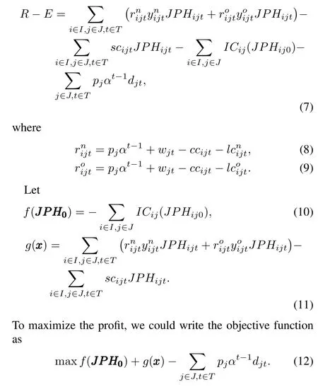
The total expense,denoted byE,is considered as the total cost plus the penalty,that is

and the pro fi t is
After combining the similar terms in(R-E),we have
Constraints
Constraints on the fi rst stage decision variables:

that is,the maximum production rates cannot be negative.
Constraints on the second stage variables are:

where:
1)Constraint(14)sets upper bounds on the actual production rates(to not let exceed the maximum production rates); 2)Constraint(15)((16),respectively)indicates that in any plant and in any period,the summation of the normal working time(overtime,respectively)of producing all the possible products cannot exceed the available total normal workingtime(total overtime,respectively)determined by the shift pattern adopted;
3)Constraint(17)indicates that no overproduction is permitted for any product in any period;
4)Constraint(18)indicates that the working time is discretely allotted to different products(unit of hours assumed).
Forclarity,wedenoteconstraints(14)~(17)by)≤0,and constraint(18)byin the following.By these denotations the formulation could be written as

This problem could not be directly solved due to the uncertainty caused by the uncertain demand.Practically,for such a stochastic problem,we usually expect to fi nd a solution ofthat is“averagely”optimal,that is,optimal in the sense of performance expectation with respect to the uncertainHence,the objective function could be written as
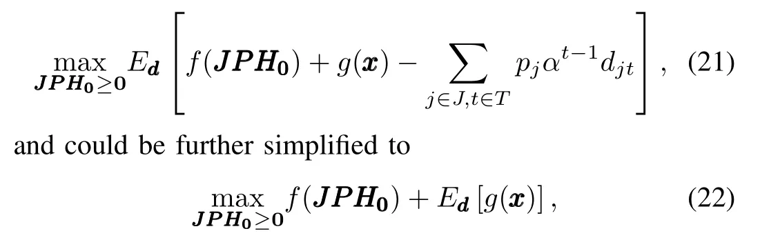
since the last term of the former is actually a constant with the distribution ofbeing known and thus has no effect on the fi nal solution and can be omitted.
For the convenience of problem analysis,we equivalently write the above formulation following the notation conventions of[9]as P1:
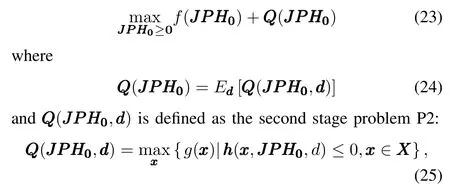
which is a deterministic programming problem trying to fi nd an optimal second stage solution with bothandbeing given.
III.PROBLEMANALYSIS ANDSOLUTION
A.Problem Complexity
To explore the complexity of P1,we fi rst analyze the complexity of the second stage problem P2.The polynomial terms in the objective functionand the constraintsmakes P2 possess no convexity and hard to be globally optimized.Furthermore,the discreteness in the normal and overtime working hours cause signi fi cant complexity in the problem.Consider a simple case of P2, which involves one plant,several products,one period,and no overtime.The number of working hours allotted to each product is constrained to be either 0 or a certain positive integer.In this case,P2 could be explicitly written as P3(with unnecessary subscripts of plant and period omitted)
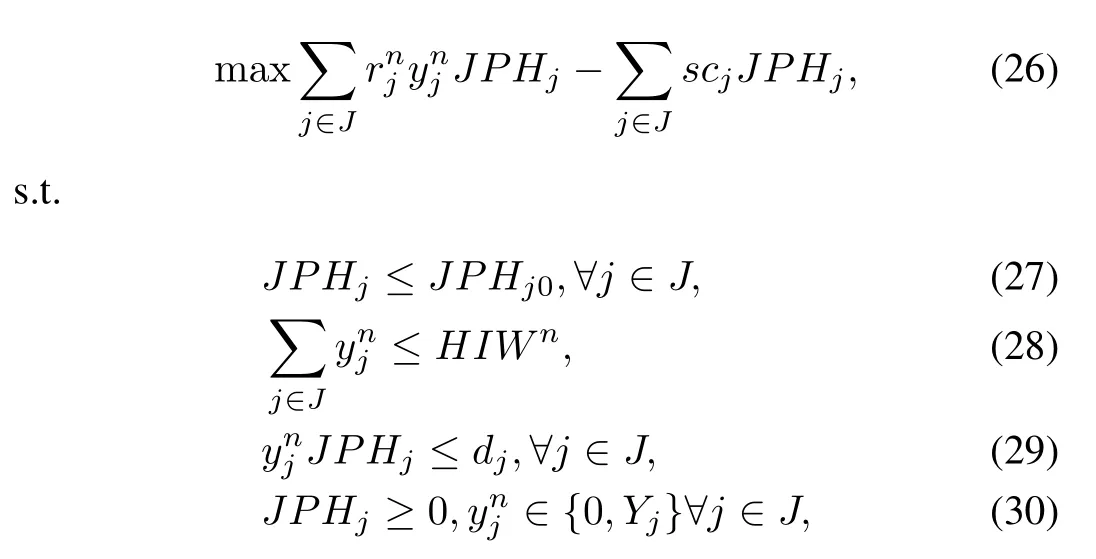
whereYjis a constant positive integer not larger thanHIWn(for anyj).We now prove P3 is NP-hard.
Proposition 1.P3 is NP-hard.
Proof.setJPHj0=dj/HIWnfor anyj∈J,which together with constraints(27)and(28)imply that,and then constraint(29)could be omitted.Furthermore,for anyj∈J,setscj=0 and=Zj·JPHj0/Yj,whereZjis a constant positive integer.Since for anyj,0,therefore the optimal solution should satisfyJPHjequals toJPHj0, and then constraint(27)could be omitted.After removal of the above restriction,we obtain a special case of problem P3 as problem P4
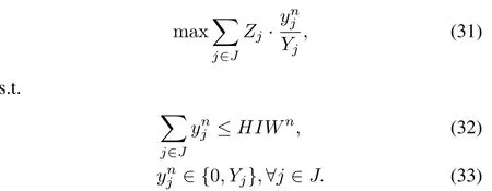
The decision version of P4 is actually a knapsack problem. Thus we know P4 is NP-hard,and so is P3.□
The whole problem P1 possesses some challenges other than the NP-hardness arising from the second stage problem P2.First,for a giventhe uncertain demandmakes the objective valuef()+)impossible to be accurately estimated.In fact,we could only estimate the expectation termbased on demand samples.That is, for a given,we generate some demand samples,solve the corresponding second stage problems with the demand samples respectively substituted for the demand variables,and then average the optimal objective values to obtainObviously,the more demand samples we use,the higher the estimation con fi dence level we would obtain,but the computation burden will correspondingly increase.
Second,the size of search space of solutions will signi ficantly increase as the size of the problem increases.Consider the case thatJPHij0could be chosen from a fi nite set withMcandidates for anyiand anyj.Then the total number of possibleisMI×J,whereIandJdenote the number of plants and number of products,respectively.We could see that the size of search space will increase exponentially with the size of the problem.
B.Solving the Second Stage Problem P2
For polynomial programming problems,there are several global optimal solution algorithms that could be found in literature.The common technique used in these algorithms is fi rst replacing the product terms with additional variables to obtain a relaxed problem and then introducing additional reasonable constraints that help to fi nd the optimal solution.One example of such algorithms is the reformulationlinearization/convexi fi cation technique(RLT)proposed in [10],being used together with branch-and-bound technique. However,RLT may not fi nd the optimal solution within fi nite steps of branch-and-bound.Another example is to convert the polynomial programming problems to 0-1 linear programming problems if the original problem possesses some special features[11].After conversion,the problem could be solved using the developed solving tools.
In our work,we converted our second stage problem to a mixed integer programming(MIP)problem by applying the conversion method proposed in[11]but with minor modi fi cation.We will fi rst introduce the converting technique fi rst and then explain the modi fi cation in the following.
Reference[11]gives an approach of converting a 0-1 polynomial programming problem to a 0-1 linear programming problem.The key idea of the approach is fi rst replacing each product term with an additional variable,and then introducing additional constraints correspondingly for each replacement such that the value of the additional variable equals to the value of the corresponding product term in any case.In this way, the two problems before and after the replacement are kept equivalent.Noting that all the polynomial terms in our problem only involve two variables,we demonstrate the approach for this case for brevity.For a polynomial programming program involving a product termu·v(u,v∈{0,1}assumed),we can substitute an additional variableWforu·v,and then introduce four additional constraints asu+v-W≤1,u≥W,v≥WandW∈{0,1}.The constraints result inW=1 only when bothuandvequal to 1 andW=0 otherwise.Thus we know the two problems before and after the substitution are equivalent.
Actually,the assumptionu,v∈{0,1}could be relaxed tou∈{0,1}andv∈[0,1],only requiring the constraintW∈{0,1}being changed toW∈[0,1]to maintain the equivalence.In this case,the constraints result inW=vwhenu=1 andW=0 whenu=0.
In our second stage problem,all the product terms involve two variables,of which one is a positive integer(or)and the other is a bounded continuous positive number (JPHijt).To apply the conversion method of[11]with the above generalization,we introduce the following substitution for anyi,jandtto make the problem contain only 0-1 integer variables and continuous variables belong to[0,1]:

where0,1}(k=1,···,K,l=1,···,L) and[0,1].The substitution and conversion result in a mixed integer programming(MIP)problem,for which we could apply any MIP solving tool,for example,the solving tool provided by IBM ILOG CPLEX[12].
C.Solving the Whole Problem P1
As discussed above,there are three main challenges to solve P1 to obtain optimal fi rst stage decisions:the NP-hardness of the second stage problem,the uncertainty of the demand and the large search space of solutions.The former two challenges determine that we could not exactly and ef fi ciently estimate the performance for a given fi rst stage decision solution.The third challenge means we have to explore a lot of candidate solutions for optimization.To meet these challenges,we turn to ordinal optimization(OO)method[8],which tries to fi nd good enough designs with a high probability instead of fi nding the optimal design for sure.OO saves computation burden by using a rough model to estimate the performance of a given design and investigate only a limited number of candidate solution sampled from the original large search space.
The OO applied solution framework for problem P1 is as follows:
Step 1.Sampling.
Randomly and uniformly sampleN(say 1000)designs of maximal production rates con fi guration().
Step 2.Performance Estimation(crude estimation).
(1)Randomly generaten1(a small number,say 1 or 2)of demand instances;
(2)For each of theNdesign samples,calculate the corresponding pro fi ts under each demand instance by solving the corresponding second stage problems,and then average the pro fi ts to obtain a rough estimation of the sample′s performance;
(3)Estimate the ordered performance curve(OPC)type based on the sorted performances of theNdesigns.
Step 3.Selecting designs(horse racing rule used here).
Order the estimated performances of the designs and select the topsdesigns as the selected set,wheresis determined according to a universal alignment probability(UAP)table and desired good enough levelk.High noise level could be assumed since no prior knowledge is known about the noise.It should be noted that the UAP adopted should conform to the required con fi dence level,i.e.,the probability of guaranteeing to fi nd a satisfactory solution later.
Step 4.Further distinguishing(more accurate performance estimation).
(1)Randomly generaten2(a relatively large number,say 10)instances of demand;
(2)Repeat the performance estimation Step 2(2)with the demand instances generated in Step4(1)to obtain more accurate estimation of the selected samples′performances;
(3)Select the design with the best average performance as the fi nal solution.
IV.NUMERICALRESULTS
A.A Numerical Example of the Second Stage Problem
To demonstrate the feasibility of the solution method of the second stage problem discussed in Section III-B,we here considered a simple example of a second stage problem,whichinvolves 2 plants,3 products and 1 period.andare given as

The normal working hours and overtime hours are respectively given as

Other coef fi cients are set such that the rewards of producing per unit of products 1 and 2 are the same,and are higher than that of producing per unit of product 3.After applying the substitution and conversion introduced in Section III-B,the resulting problem could be solved by ILOG CPLEX and an optimal solution could be obtained as:
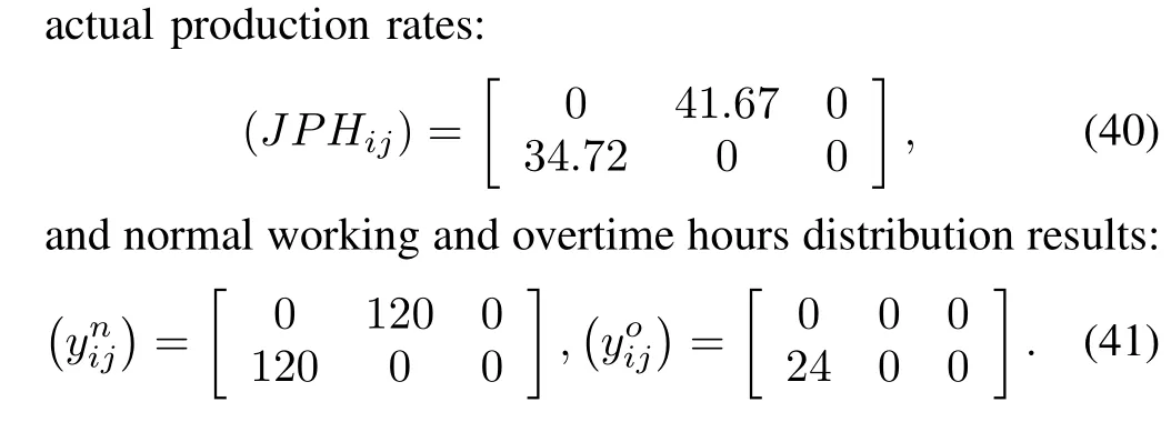
The results are reasonable in the sense that the production time are allotted to more pro fi table products(products 1 and 2)other than the less pro fi table product(product 3).
B.A Numerical Example of the Whole Problem P3
We considered an example of vehicle manufacturing system. The system is composed of 10 plants,and is built to produce 5 models of vehicles in a decision horizon of 520 periods (10 years).Of the fi ve vehicle models,two are assumed to be popular through the decision horizon and the demands of them are relatively steady without much variance.The other three are assumed to be new models that are coming into the market at the beginning of the decision horizon,the beginning of the second year and the beginning of the third year,respectively.Their life time is assumed to be about 10 years.The demands of these three models are assumed to follow a Bass model[13],which sequentially increases,reaches its peak,and then decreases.The cumulative quantity of a Bass model quantity fi ts an S-shape curve.
We assumed 0≤JPHij0≤50,for anyiand anyj. Other given values are too many to be listed here and thus are omitted.
The problem was solved following the steps of the solution framework given in Section III-C.One run of the solution process was as follows:
Step 1.One thousand samples ofwere uniformly and randomly generated.
Step 2.As a rough estimation of the samples′performance, we respectively calculated the samples′corresponding pro fi ts under one randomly generated demand instance.The normalized OPC was then obtained based on the sorted performances.
Step 3.It is calculated that the selected set should contain at least 30 designs to ensure with probability 0.95 that the selected set contains at least one actual top 5%design.Thus the top 30 samples of the sorted are chosen as the selected set.
Step 4.To gain more accurate estimation of the selected samples′performances so as to further distinguish them,we calculated their respective average pro fi t under 10 randomly generated demand instances,and chose the design with the highest average pro fi t as the fi nal solution.
In Steps 2 and 4,the demand instances of the 5 vehicle models in the 10 years are generated as follows.For those two popular models,their demands are respectively generated randomly and uniformly within a given range.For those three that fi t Bass model,the demands are generated based on the Bass model formula but with random noises injected into them. One example instance is given as Fig.5.

Fig.5.An example of generated demand instances.
The result of Step 2 shows that with the crude performance estimation the pro fi t corresponding to the sorted best design is 17.3%higher than that corresponding to the sorted worst one.This well indicates that a proper design ofcould make signi fi cant performance improvement and that one can actually achieve such improvement with optimization.The normalized OPC obtained in Step 2 is shown in Fig.6,which fi ts a bell type OPC de fi ned in OO theory,indicating that there are relatively few good designs,many intermediate and few bad designs(the rightmost and leftmost segments of the curve are steep).The fi nal solution distinguished in Step 4 is shown in Table I.
To evaluate the performance of the fi nal solution,we compared its performance to all the other sampled designs and other 9,000 randomly and uniformly sampled designs with a more accurate performance estimation model,namely,to see how good the fi nal solution′s performance is among a total number of 10000 randomly and uniformly sampled designs. The result shows that the performance of the fi nal solution ranks 242 in all the sampled designs,belonging to the top 5% good enough solution set.This indicates that the OO algorithm indeed found a satisfactory solution.Furthermore,we obtained another OPC with the 10000 designs′sorted performances(as showed in Fig.7).This OPC is believed to better approximate the true OPC compared to the one showed in Fig.6 since a relatively large number of designs are investigated here with the more accurate performance estimation model.Because the true OPC of the problem cannot be obtained due to the problem complexity analyzed in Section III-A,practically this OPC can be seen as a quasi-true OPC of the problem.From Fig.6 and Fig.7 we can see the estimated OPC obtained in Step 2 is of the same type as the quasi-true OPC.Thus weknow the 1000 designs sampled in Step 1 above can actually be a representation of the original search space and the OO method is rational to be applied to this problem.
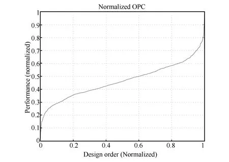
Fig.6.The normalized OPC of the numerical example in Section IV-B(1000 sampled designs,rough performance estimation model).

Fig.7.The quasi-true OPC of the numerical example in Section IVB(10000 sampled designs,more accurate performance estimation model)).
To gain a rough idea of the performance of the OO algorithm,we run the solution process for 10 replications as above and checked the performance of the fi nal solution for each replication.The result shows that all of 10 runs fi nd a fi nal solution that is satisfactorily among the top 5%.This demonstrates the OO algorithm′s feature of guaranteeing a high probability of fi nding satisfactory solutions.It should be noted that this validation step is not necessary in practical use.
V.CONCLUSION
The planning model we proposed in this paper is important to help the decision making on the investment on the production lines to best balance between meeting the future demand and saving cost,and thus obtaining the maximum pro fi t in the planning horizon.The challenge is the complex nature of the problem which makes the solution dif fi cult to obtain For a given design,the uncertainty in demand makes the exact performance estimation impossible.If we require the estimation has a high con fi dence level,the computation burden would be signi fi cantly high.The OO method allows a rough model to estimate the performance of designs and only requires looking into a relatively small number of designs,and thus could be applied to our problem with notable reduction of the computation burden.This modeling framework and the optimization concept could provide helpful insights for similar scenario applications.

TABLE I FINAL SOLUTION OF THE NUMERICAL EXAMPLE
It should be pointed out that when determining which candidate solution can be selected as the fi nal solution,more advanced methods,such as optimal computing budget allocation(OCBA)[14],could be applied to further enhance the ef fi ciency of the solution framework.However,this is beyond the scope of this paper and is to be explored in our future work.
REFERENCES
[1]Fleischmann B,Ferber S,Henrich P.Strategic planning of BMW′s global production network.Interfaces,2006,36(3):194-208
[2]Kauder S,Meyr H.Strategic network planning for an international automotive manufacturer:balancing fl exibility and economical ef fi ciency.OR Spectrum,2009,31(3):507-532
[3]Bihlmaier R,Koberstein A,Obst R.Modeling and optimizing of strategic and tactical production planning in the automotive industry under uncertainty.OR Spectrum,2009,31(2):311-336
[4]Lin J T,Wu C H,Chen T L,Shih S H.A stochastic programming model for strategic capacity planning in thin fi lm transistor-liquid crystal display(TFT-LCD)industry.Computers&Operations Research,2011, 38(7):992-1007
[5]Zhang R Q,Zhang L K,Xiao Y Y,Kaku I.The activity-based aggregate production planning with capacity expansion in manufacturing systems.Computers&Industrial Engineering,2012,62(2):491-503
[6]Kulkarni A A,Shanbhag U V.Recourse-based stochastic nonlinear programming:properties and benders-SQP algorithms.Computational Optimization and Applications,2012,51(1):77-123
[7]Chien C F,Wu J Z,Wu C C.A two-stage stochastic programming approach for new tape-out allocation decisions for demand ful fi llment planning in semiconductor manufacturing.Flexible Services and Manufacturing Journal,2013,25(3):286-309
[8]Ho Y C,Zhao Q C,Jia Q S.Ordinal Optimization:Soft Optimization for Hard Problems.New York:Springer,2007.
[9]Birge J R,Louveaux F.Introduction to Stochastic Programming.New York:Springer,1997.
[10]Sherali H D,Tuncbilek C H.A global optimization algorithm for polynomial programming problems using a reformulation-linearization technique.Journal of Global Optimization,1992,2(1):101-112
[11]Glover F,Woolsey E.Converting the 0-1 polynomial programming problem to a 0-1 linear program.Operations Research,1974,22(1): 180-182
[12]IBM ILOG CPLEX.ILOG CPLEX 11.0 User′s Manual.France,2007.
[13]Bass F M.A new product growth for model consumer durables.Management Science,1969,15(5):215-227
[14]Chen C H,Lin J W,Yu¨cesan E,Chick S E.Simulation budget allocation for further enhancing the ef fi ciency of ordinal optimization.Discrete Event Dynamic Systems,2000,10(3):251-270


Qianchuan Zhao Professor and associate director of the Center for Intelligent and Networked Systems(CFINS)in the Department of Automation, Tsinghua University.His research interests include performance optimization and security control for networked dynamical systems.Corresponding author of this paper.

Ningjian Huang is a group manager at Manufacturing Systems Research Lab,Global R&D Center,General Motors Company.He received his Ph.D.degree in Systems Engineering from Oakland University in 1991.He joined GM the same year, and has worked on numerous research projects in manufacturing related areas.His current job capacity includes portfolio management for GM global advance manufacturing projects and leading role of manufacturing fl exibility,production control and management.His research interests include manufacturing system modeling,simulation,analysis and optimization.

Xiang Zhao received the Ph.D.degree in mechanical engineering.He started his automotive career in 1994.He joined GM vehicle operation organization in 1998 as a senior project engineer,and promoted to staff engineer in 2002.From 2004 to 2005,he worked as cost reduction manager in GM global luxury RWD vehicle line team.from 2006 to 2007, he worked as new business development manager in GM global purchasing and supply Chain organization.Since 2008,he has been working as staff researcher in Manufacturing Systems Research Lab at GM Global R&D.
Over past 20 years,he has worked in various engineering/technical/-management fi elds ranging from manufacturing system/process validation, simulation,and testing/analysis,sustainable manufacturing system and supply chain research,to supplier footprint strategy planning/optimization and manufacturing R&D strategy planning.Through his work in GM′s global cross-functional teams and various organizations,he gained valuable indepth knowledge and experience in GM′s vehicle program planning and management,global procurement process,supply chain development and manufacturing engineering and R&D.
Xiang Zhao served as Society of Manufacturing Engineers(SME)founding chapter(Chapter One)Chairman in 2002,SME Great Lakes Region Public Relation Committee Chairman in 2003,SME Production Systems and Management Techniques Technical Committee member from 2002 to 2004.
eceived his bachelor and Ph.D.degrees from Tsinghua University in 2008 and 2014,respectively.He has joined the Institute of Space System Engineering,China Academy of Space Technology since August 2014.His research interests include simulation-based performance estimation and optimization for large-scale complex stochastic systems.
Manuscript
September 12,2012;accepted January 29,2013. This work was supported by a contract between General Motors Company and Tsinghua University,National Natural Science Foundation of China (61425027,60736027,61021063,61074034,61174105).Recommended by Associate Editor Shiji Song.
:Hao Liu,Qianchuan Zhao,Ningjian Huang,Xiang Zhao.Production line capacity planning concerning uncertain demands for a class of manufacturing systems with multiple products.IEEE/CAA Journal of Automatica Sinica,2015,2(2):217-225
Hao Liu is with the Center for Intelligent and Networked Systems(CFINS), Department of Automation,TNList Lab,Tsinghua University,Beijing 100084, China,and also with the Research and Development Center,Institute of Space System Engineering,China Academy of Space Technology,Beijing 100094, China(e-mail:hiliuhao@163.com).
Qianchuan Zhao is with the Center for Intelligent and Networked Systems (CFINS),Department of Automation,TNList Lab,Tsinghua University, Beijing 100084,China(e-mail:zhaoqc@tsinghua.edu.cn).
Ningjian Huang and Xiang Zhao are with the Global Research and Development Center,General Motors Company,Warren,MI 48090,USA(email:ninja.huang@gm.com;xiang.zhao@gm.com).
 IEEE/CAA Journal of Automatica Sinica2015年2期
- IEEE/CAA Journal of Automatica Sinica的其它文章
- Single Image Fog Removal Based on Local Extrema
- An Overview of Research in Distributed Attitude Coordination Control
- Operation Ef fi ciency Optimisation Modelling and Application of Model Predictive Control
- Cloud Control Systems
- Stable Estimation of Horizontal Velocity for Planetary Lander with Motion Constraints
- Consensus Seeking for Discrete-time Multi-agent Systems with Communication Delay