The Selective Control Feature for Physically Accurate Solutions of All Variables and Application in First Order Linear Transient Hyperbolic Systems

S.Masuri,and K.K.Tamma

1 Introduction

Numerical simulations typical of first order hyperbolic systems requires robust computational methods that also possess controllable numerical dissipative features to meet the strict needs in integrating such problems for very long time periods to obtain physically accurate solutions,i.e.,solutions that correctly capture the dynamics of the problem.This is due to the unrealistic behavior of numerically nondissipative schemes such as the Crank-Nicolson method by Crank and Nicolson(1947)which often yield numerical solutions that switch sign on each step due to their zero damping property regardless of the time step.Such behavior can cause non-physical instabilities and in some cases can lead to the non-convergence of the nonlinear iteration during a typical time step.This problem can be successfully treated by damping the high temporal frequencies which can be achieved by introducing controllable numerical dissipation in the computational method.

Controllable numerical dissipative methods including optimal algorithm designs exist for integrating second order dynamic systems such as elastodynamics problems,and to a limited extent have also been applied to first order systems for integrating the transient system of equations by Zhou and Tamma(2004,2006);Masuri,Sellier,Zhou,and Tamma(2011);K.E.Jansen et.al(2000).Recently,we have described a generalized single-system single-solve computational approach that permits algorithms with second order time accurate features,and unconditionally stability with zero order overshoot behavior for a family of time for the integration of transient first order parabolic systems such as the heat conduction type,termed as GS4-1 framework by Masuri,Sellier,Zhou,and Tamma(2011).Such a family of methods were developed by utilizing in a consistent manner the design procedure previously introduced for second order systems via a generalized time weighted residual approach,and referred to asAlgorithms by Designby Zhou and Tamma(2004,2006).In our previous exposition in Masuri,Sellier,Zhou,and Tamma(2011),we illustrated the design and development of this framework and provided validation using a benchmark first order parabolic heat conduction type problem where we assessed the efficiency and accuracy of the developed framework.

The key feature in this framework is the incorporation of a spurious root(ρs∞),in addition to the principal root(ρ∞),to allow for selective and more flexible control of the high frequency damping(for both the primary variable and its time derivative,respectively)for a successful simultaneous elimination of the numerical oscillation associated with these variables.Such a design thereby yields a two-parameter(ρ∞and ρs∞)family of methods with a more flexible user control of high frequency damping for the two variables,respectively.The one-parameter time integrator is a particular case recovered by allowing the two parameters to be equal(i.e,ρ∞=ρs∞),in which case the amount of the high frequency damping for the two variables is hence equal.However,the same amount of damping may not be sufficient to suppress the numerical oscillation in the time derivative variable.To overcome this drawback,we allow a more flexible control of the high frequency damping by introducing different amounts of numerical dissipation in the two variables which is inherent in the present developments.Such a selective control of the high frequency damping would allow simultaneous elimination of the numerical oscillation associated with the two variables,leading to physically accurate solutions of these variables.This feature is hereby termed as the “selective control feature”.

In this paper,our objective is to extend the GS4-1 framework from applications in parabolic type situation to hyperbolic type applications pertaining to first order linear transient systems,that frequently arise in flow transport phenomena and transport of heat in moving media.Whilst the focus in Masuri,Sellier,Zhou,and

Tamma(2011)was on the detailed design of the GS4-1 framework and provide validation in a general sense;in this paper,attention is paid to describe in more details the new selective control feature,which is the crux of the present framework,and discuss the effects and role played by this new feature in generating physically accurate solutions of all variables in the system.In this work,whilst on one hand we show that an equal amount of high frequency damping(i.e,without the selective control feature:ρ∞=ρs∞)leads to non-physical instability in the time derivative variable for a minimal damping required to obtain acceptable solution of the primary variable;on the other hand,we particularly demonstrate how this instability can be easily turned off via the selective control feature(i.e,ρ∞/=ρs∞)offered by our developed framework,thereby,demonstrating its robustness and superiority.The outline of the paper is as follows:In Section 2 we briefly review the formulation of spatial discretization of the time dependent first order hyperbolic problems using the Finite Element Method.This is followed by the formulation of the GS4-1 framework due to Masuri,Sellier,Zhou,and Tamma(2011)which is extended to first order hyperbolic systems in this paper to discretize the temporal domain in Section 3.We then demonstrate the advantages of GS4-1 computational framework with the selective control feature by solving two numerical examples as described in Section 4.Finally,conclusions are drawn and presented in Section 5.

2 Governing Equations and Spatial Discretization

Consider for illustration,the linear transient first order hyperbolic system of the following form

with conditions on the boundary Γ as

and initial condition

where φ(x,t)is the primary variable at position x and timet,v is the velocity vector,κ is the constant diffusion coefficient,x=(x1,x2,....,xd)is the vector position,dis the dimension of the problem,Ω is a bounded domain inRd,Γ is the boundary on Ω,and φΓ(x,t),q(x),and φ0are known vectors of boundary and initial conditions.

Equation(1)can be nondimensionalized by introducing dimensionless primary variablevelocitytimeand coordinatewhereLis the specific length of the domain,Uis the characteristic velocity of the flow,while φref1and φref2are the lower and upper reference values of the primary variables,respectively.From the use of these dimensionanless variables,equation(1)can be represented in dimensionless form as follows

whereWis the weighting function and Ω(e)is the domain for an element(e).We next apply Gauss’s theorem to the diffusion term to yield

We next approximate the primary variable φ(x,t)as follows

whereN(x)is the element shape function and φ(t)is the vector of nodal solutions of the element at timet.Substituting equation(9)into equation(8)and imposing the Neumann boundary condition(equation(3))yield the following first order ordinary differential equation system

where

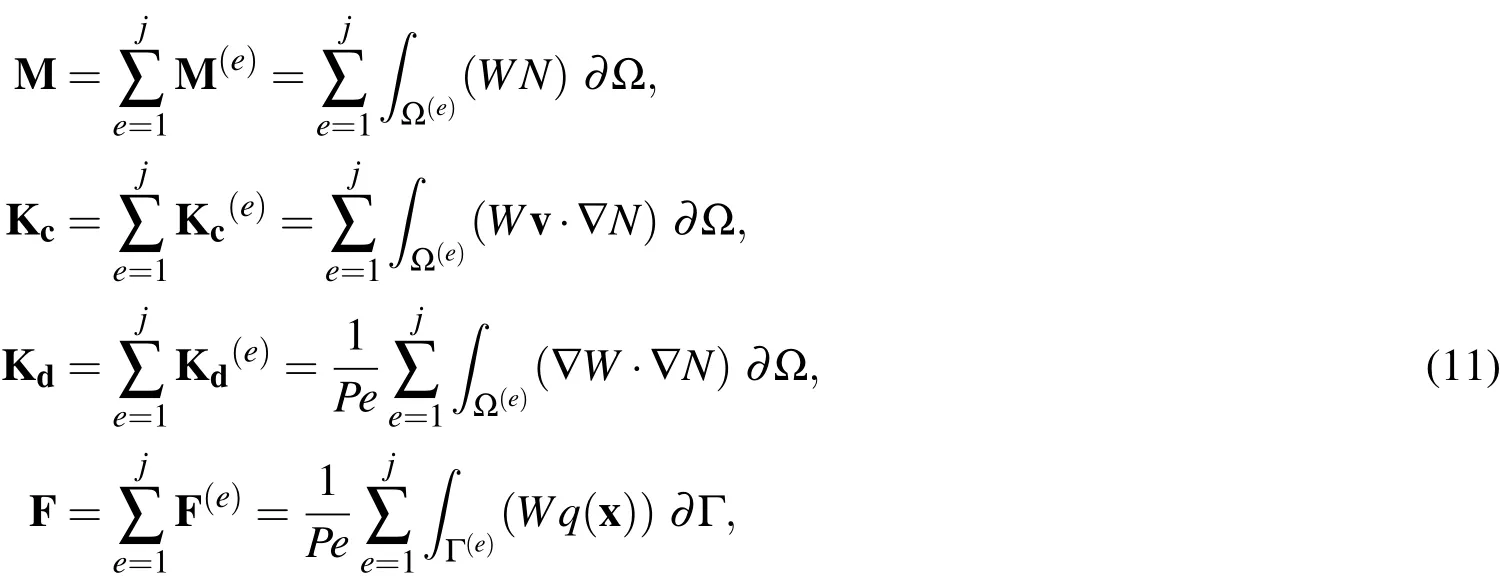
are the mass matrix,stiffness matrix due to convection,stiffness matrix due to diffusion,and force vector due to the Neumann boundary condition,respectively,whilejis the total number of elements used in the spatial discretization.

3 Time Integration by GS4-1 Computational Framework

We proceed in this section by presenting how the GS4-1 computational framework can be adapted for use in first order transient hyperbolic systems,in particular for the integration of equation(10)fromtntotn+1(i.e.,Δt=tn+1−tn)(detailed derivation and development of the framework has been presented in Masuri,Sellier,Zhou,and Tamma(2011),with particular application to parabolic system,and therefore will not be repeated here).

Equation(10)can be integrated fromtntotn+1using the GS4-1 framework as follows:Given the solutions attntime level(φnand),we first solve for φn+1from

and followed by updating the time derivative variable()as follows

where ρ∞andare the two,user-defined parameters,satisfying the following conditions in Masuri,Sellier,Zhou,and Tamma(2011)

3.1 The Selective Control Feature

The selective control feature,which is new and is not available in any existing methods to-date,can be achieved by definingso long as the condition that 0≤≤ρ∞≤1 is satisfied.On the other hand,by defining ρ∞=,the selective control feature is turned off and the framework recovers existing method without such feature in K.E.Jansen et.al(2000).The underlying physical interpretations of the feature is the following(see Masuri,Sellier,Zhou,and Tamma(2011)for details):the two parameters separately control the high frequency damping of the primary variable(φ)and its time derivative(),respectively.That is,ρ∞is associated with the numerical dissipative property of φ.If ρ∞=1,the resulting algorithm is said to impose no numerical dissipation on φ(i.e.,zero-damping).On the other hand,ρ∞=0 means that the algorithm imposes maximal numerical damping on φ.Meanwhile,is associated with the numerical dissipative property of,and likewise,=1 means that no numerical dissipation is imposed onwhile=0 indicates that maximal numerical dissipation is imposed on this variable.

The new selective control feature allows for different amounts of numerical dissipation in φ andby choosingto obtain successful simultaneous elimination of the numerical oscillations associated with these two variables.This is in contrast to the past development in which the numerical dissipations of these two variables are of limited control,often indiscriminately(i.e.,ρ∞=),causing numerical instabilities in the time derivative variable which has practical importance as evidenced from literature in Belmonte and Libchaber(1996);Schroers,Masuhr,Johnson,and Busch(1999).Other related works in flow problems appear in Golberg and Chen(2011),Lin and Atluri(2001),Nicolas and Bermudez(2004),Selvadurai and Dong(2006),and Mohammadi(2008).The present developments instead yield a two-parameter(ρ∞and)family of methods with a more flexible user control of high frequency damping for the two variables.Equally important is the fact that we are able to introduce this new feature while preserving second order accuracy(i.e.,order preserving feature)resulting in a 2-root system.This is in contrast to the classical Trapezoidal family of algorithms which is only a single root system.

4 Numerical Examples and Validation

In this section,we will provide validations on the importance of the selective control feature available in the GS4-1 framework for applications typical of hyperbolic type pertaining to first order transient system.For this purpose,we consider two numerical examples in one-and two-dimensional applications governed by a linear transient convection-diffusion equation.

4.1 1D Problem

The simplicity of the problem eliminates any need for upwinding in the spatial discretization unlike the next example to follow.Therefore,this example will provide real comparison of the GS4-1 computational framework with and without the selective control feature without any effect of upwinding on the solutions.The problem has the following initial and boundary conditions

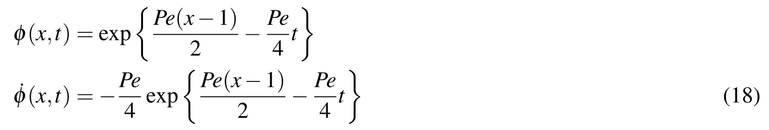
where the analytical solution is Grigoriev and Dargush(2003)given by

The problem parameters in nondimensional form used are:v=1 andPe=0.1.For this problem,we use 1D linear elements,whose element shape functions are given by

wherelis the length of each element.We discretize the spatial domain using 50 elements to yield a cell Peclet number of 0.002,in which case the Bubnov-Galerkin FEM can be appropriately used.In this method,the weighting function in equation(11)takes similar form of the element shape function(i.e.,W=N)given by equation(19).We substitute this equation into equation(11)and sum for each element to form global matrices in equation(10).

We recall that the one-parameter time integrator is a particular case recovered in the GS4-1 framework by defining ρ∞=(i.e.,the case without the selective control feature).To demonstrate the importance and role played by the selective control feature,in contrast to existing method without such feature),we solve the problem using the GS4-1 framework with two cases(i.e.,with and without the selective control feature)with a dimensionless time step size Δt=2 and a dimensionless end timet=20.While having two parameters(ρ∞and)in the GS4-1 framework has a certain appeal,we recall that our aim is to simultaneously suppress the nonphysical instabilities in both φ andto obtain solutions that are not only acceptable but also represent the correct dynamics of the problem.For this purpose,we lettake a zero value regardless of the value of ρ∞.Not only that this will ensure a successful elimination of the numerical oscillation associated with,such an approach would also allow for widest range of ρ∞to be tested(due to the restriction that 0≤≤ρ∞≤1).Given this constraint onvalue,the GS4-1 framework has only one parameter left to be specified(i.e.,ρ∞).For comparison purposes,we choose ρ∞for the case without the selective control feature to take the same value as the ρ∞for the case with such feature.The ρ∞values may range from 1(i.e.,nondissipative/zero damping)to 0(i.e.,maximal damping).

妈妈说：快要卸货的我心里有几分激动，这是计划中的最后一次产检，我期待着一切顺利，可检查完被妇产科医生告知：孩子头太大，骨盆太窄，有些头盆不称，建议我剖宫产。一直坚持顺产的我听到如此消息后，最关心的就是剖宫产会在肚子上切一刀，这个切口有多长，是横切还是竖切？术后该如何护理，有疤痕怎么办？

Figure 4 shows the plots of nondimensional φ andas a function of nondimensional time for node number2(x=0.02)as generatedby the GS4-1 framework with and without selective control feature for ρ∞=0.8.Meanwhile,Figure 3 shows the plots of analytical solutions(both nondimensional φ andas given by equation(18))as a function of nondimensional time for this node.We can see from Figure 4 that both cases yield good results for the primary variable.However,for the time derivative variable(),the case without the selective control feature results in large oscillation.This representation(i.e.,method without the selective control feature)controls the numerical damping of both the nondimensional φ andindiscriminately;hence,a ρ∞value of 0.8 means a correspondingvalue of 0.8 as well.It is demonstrated from this figure thatrequires more numerical damping than this value for a physically accurate solution.This can be easily achieved when the selective control feature is turned on,to yield good agreement with the analytical solution with the same ρ∞value.By allowing thevalue to take on zero value via the selective control feature,sufficient numerical damping is given to the time derivative variable()such that the large oscillation is successfully eliminated.This demonstrates the importance and roles played by the new selective control feature to yield physically accurate solutions of both the primary variable and its time derivative,enabling the physics and dynamics of the problem to be correctly captured.Figure 7 shows the plots of analytical solutions of nondimensional φ andas given by equation(18))as a function of the spatial domain at a specific nondimensional timet=20.Meanwhile,Figure 8 shows the numerical results generated by the two cases for ρ∞=0.8.From this figure,we can see that the same observations as those seen in Figure 4 are repeated here,i.e.,(1)that both cases yield good results for φ,(2)that the case without the selective control feature results in large oscillation for,and(3)that the GS4-1 framework with the selective control feature could yield good agreement with the analytical solution with the same ρ∞value,in contrast to the case without such feature This,again,illustrates the importance of and the role played by the new feature introduced in the GS4-1 framework,which is the selective control of the high frequency damping for all variables.

Figure 1:Plot of analytical solutions of solutions nondimensional φ and as a function of nondimensional time for node number 2(1D problem)as given by equation(18)

We next compute and compare the errors in nondimensional φ andgenerated by these two representations for a given set of ρ∞value ranging from 1(nondissipative/zero numerical damping)to 0(maximal numerical damping)in a decrement of 0.1 for completion of the investigation.The error is defined as

Figure 2:Plot of nondimensional φ and as a function of nondimensional time for node number 2(1D problem)generated by:(i)GS4-1(ρ∞=0.8,=0),and(ii)GS4-1(ρ∞=0.8,=0.8),i.e.,the case without selective control features

Table 1 first shows the comparison of maximal and total errors in the primary variable(φ)between the cases involving features with and without selective control of the high frequency damping of the primary variable and its time derivative for all ρ∞values considered.For the small amount of dissipation(0.7≤ρ∞≤1)that is desirable,the GS4-1 framework with the selective control feature yields slightly better results than the one without such feature.For larger amount of controllable numerical dissipation(0≤ρ∞≤0.7),an opposite trend is observed.However,it is to be noted that the results generated by the two cases are on the same order of magnitude which is small(x10−7).Therefore,we conclude that both cases perform well to suppress the numerical oscillation associated with the primary variable(φ).Alternately,Table 2 next shows the comparison of maximal and total errors in the time derivative variable()between the two cases.In this table,the difference in performance between the two different representations is obvious.The case without the selective control yields large errors(both maximal and total)for almost all ρ∞values considered with exception for large amount of dissipation(0≤ρ∞≤0.2).These large errors indicate that this representation(i.e.,the case without selective control)is not capable of eliminating the numerical oscillation associated withfor the given amount of damping.On the other hand,when the selective control feature is turned on,the error inis reduced to an acceptable level(x10−6for maximal error and x10−5for total error)for all ρ∞values considered.This,again,highlights the importance of the selective control feature.

Figure 3:Plot of analytical solutions of solutions nondimensional φ and as a function of nondimensional time for node number 2(1D problem)as given by equation(18)

Figure 4:Plot of nondimensional φ and as a function of nondimensional time for node number 2(1D problem)generated by:(i)GS4-1(ρ∞=0.8,=0),and(ii)GS4-1(ρ∞=0.8,=0.8),i.e.,the case without selective control features

Figure 5:Plot of analytical solutions of nondimensional φ and as a function of x at a specific nondimensional time t=20(1D problem)as given by equation(18)

4.2 2D Problem

This higher dimensional problem serves to further provide a consistent observation for the two-dimensional case as well.The problem is defined in dimensionless form as follows:

with the following Dirichlet type boundary and initial conditions

Figure 6:Plot of nondimensional φ and as a function of x at a specific nondimensional time t=20(1D problem)generated by:(i)GS4-1(ρ∞=0.8,=0),and(ii)GS4-1(ρ∞=0.8=0.8),i.e.,the case without selective control features

where the analytical solution is given by Durmus,Boztosun,and Yasuk(2006)

The constant physical properties and problem parameters in dimensionless form used are:vx=vy=10,Pe=10,a=1,andb=0.1.For this problem,we use 2D linear elements of width 2band height 2hwhose element shape functions are given

Figure 7:Plot of analytical solutions of nondimensional φ and as a function of x at a specific nondimensional time t=20(1D problem)as given by equation(18).

Table 1:Comparison of error in φ for the 1D problem between:(i)the case without selective control with ρ∞ = ρ∞,and(ii)the GS4-1 framework with selective control features with =0,for ρ∞values ranging from 1(zero damping)to 0(maximal damping)in decrements of 0.1.

Table 1:Comparison of error in φ for the 1D problem between:(i)the case without selective control with ρ∞ = ρ∞,and(ii)the GS4-1 framework with selective control features with =0,for ρ∞values ranging from 1(zero damping)to 0(maximal damping)in decrements of 0.1.

ρ∞Max Error Total Error Without selective control selective control Without selective control selective control 1 3.9843x10−8 3.9843x10−8 1.1475x10−6 1.1475x10−6 0.9 4.2057x10−7 3.8863x10−7 1.4304x10−5 1.3424x10−5 0.8 5.2262x10−7 3.5253x10−7 1.8027x10−5 1.2157x10−5 0.7 3.6626x10−7 2.9354x10−7 1.2729x10−5 1.0041x10−5 0.6 2.3980x10−7 2.8144x10−7 8.3074x10−6 9.5509x10−6 0.5 2.0673x10−7 3.0492x10−7 7.0651x10−6 1.0305x10−5 0.4 2.2992x10−7 3.4643x10−7 7.7878x10−6 1.1690x10−5 0.3 2.7970x10−7 3.9812x10−7 9.4465x10−6 1.3426x10−5 0.2 3.5293x10−7 4.5924x10−7 1.1906x10−5 1.5481x10−5 0.1 4.6029x10−7 5.3200x10−7 1.5516x10−5 1.7927x10−5 0 6.2006x10−7 6.2006x10−7 2.0887x10−5 2.0887x10−5

Figure 8:Plot of nondimensional φ and as a function of x at a specific nondimensional time t=20(1D problem)generated by:(i)GS4-1(ρ∞=0.8,=0),and(ii)GS4-1(ρ∞=0.8,=0.8),i.e.,the case without selective control features.

by

Table 2:Comparison of error in for the 1D problem between:(i)the case without selective control with ρ∞ = ρ∞,and(ii)the GS4-1 framework with selective control features with=0,for ρ∞values ranging from 1(zero damping)to 0(maximal damping)in decrements of 0.1.

Table 2:Comparison of error in for the 1D problem between:(i)the case without selective control with ρ∞ = ρ∞,and(ii)the GS4-1 framework with selective control features with=0,for ρ∞values ranging from 1(zero damping)to 0(maximal damping)in decrements of 0.1.

ρ∞Max Error Total Error Without selective control selective control Without selective control selective control 1 82.3789 1.5406x10−6 112.5317 7.6500x10−5 0.9 28.7237 1.8570x10−6 39.2378 8.8870x10−5 0.8 8.8454 1.7989x10−6 12.0832 8.6881x10−5 0.7 2.3270 1.6990x10−6 3.1789 8.3390x10−5 0.6 0.4981 1.6409x10−6 0.6805 8.1343x10−5 0.5 0.0805 1.6181x10−6 0.1100 8.0536x10−5 0.4 0.0086 1.6115x10−6 0.0119 8.0298x10−5 0.3 4.8819x10−4 1.6094x10−6 7.4774x10−4 8.0224x10−5 0.2 9.4825x10−6 1.6078x10−6 6.4129x10−5 8.0169x10−5 0.1 2.0424x10−8 1.6059x10−6 8.3418x10−7 8.0107x10−5 0 1.6036x10−6 1.6036x10−6 8.0031x10−5 8.0031x10−5

We substitute equation(24)and(25)into equation(11)and sum for each element to form global matrices in equation(10).

We solve the problem using the two cases with a nondimensional time step size Δt=1 and a nondimensional end timet=20 with ρ∞=0.8 and show the numerical results for node number 25(x=0.05,y=0.15)as a function of nondimensional time in Figure 12.Meanwhile,the analytical solutions,as given by equation(23),are shown in Figure 11.Figure 12 shows that both representations yield good results for φ.However,the case without selective control feature results in large numerical oscillation for the time derivative variable().The GS4-1 framework with selective control features,on the other hand,could yield physically accurate results with good agreement to the analytical solution with the same ρ∞value.

Figure 9:Plot of analytical solutions of nondimensional φ and as a function of nondimensional time for node number 25(2D Problem)as given by equation(23).

Figure 10:Plot of nondimensional φ and as a function of nondimensional time for node number 25(2D Problem)generated by:(i)GS4-1(ρ∞=0.8,=0),and(ii)GS4-1(ρ∞=0.8,=0.8),i.e.,the case without selective control features.

Figure 11:Plot of analytical solutions of nondimensional φ and as a function of nondimensional time for node number 25(2D Problem)as given by equation(23)

Figure 12:Plot of nondimensional φ and as a function of nondimensional time for node number 25(2D Problem)generated by:(i)GS4-1(ρ∞=0.8,=0),and(ii)GS4-1(ρ∞=0.8,=0.8),i.e.,the case without selective control features

We repeat the same procedure to determine error of nondimensional φ andas previously done in the 1D problem and show the results in Table 3 and 4.An observation from Table 3 indicates that the error in φ generated by the two distinctly different representations are the same order of magnitude and are small(10−5for maximal error and 10−3for total error).Therefore,we conclude that both the GS4-1 framework involving features with and without selective control of the high frequency damping of the primary variable and its time derivative work well to obtain acceptable solutions of φ.This conclusion is similar to that found in the 1D problem.However,on the other hand,the errors in(both maximal and total)generated by the case without selective control features are large as seen in Table 4,except for large amount of damping(0≤ρ∞≤0.5)that is less desirable.These errors are significantly reduced to acceptable level(10−4for maximal error and 10−2for total error)when the selective control feature is turned on.It is hence apparent that the previous observations are repeated in this two-dimensional case.This provides validation on the consistency of the argument;that the selective control feature,which is new and not available in existing methods to-date for first order transient system,plays important roles to yield physically accurate solutions of all variables involved in the system that is important to correctly capture the physics and dynamics of the problem.

Table 3:Comparison of error in φ for the 2D Problem between:(i)the case without selective control features with ρ∞ = ρ∞,and(ii)GS4-1 framework with selective control features with=0,for ρ∞values ranging from 1(zero damping)to 0(maximal damping)in decrements of 0.1.

Table 3:Comparison of error in φ for the 2D Problem between:(i)the case without selective control features with ρ∞ = ρ∞,and(ii)GS4-1 framework with selective control features with=0,for ρ∞values ranging from 1(zero damping)to 0(maximal damping)in decrements of 0.1.

ρ∞Max Error Total Error Without selective control selective control Without selective control selective control 1 7.7101x10−5 7.7101x10−5 0.0014 0.0014 0.9 8.2838x10−5 8.4817x10−5 0.0015 0.0015 0.8 8.5482x10−5 8.5802x10−5 0.0015 0.0015 0.7 8.5896x10−5 8.5883x10−5 0.0015 0.0015 0.6 8.5925x10−5 8.5866x10−5 0.0015 0.0015 0.5 8.5911x10−5 8.5840x10−5 0.0015 0.0015 0.4 8.5887x10−5 8.5810x10−5 0.0015 0.0015 0.3 8.5853x10−5 8.5775x10−5 0.0015 0.0015 0.2 8.5804x10−5 8.5736x10−5 0.0015 0.0015 0.1 8.5735x10−5 8.5689x10−5 0.0015 0.0015 0 8.5635x10−5 8.5635x10−5 0.0015 0.0015

Table 4:Comparison of error in for the 2D Problem between:(i)the case without selective control features with ρ∞ = ρ∞,and(ii)GS4-1 framework with selective control features with=0,for ρ∞values ranging from 1(zero damping)to 0(maximal damping)in decrements of 0.1.

Table 4:Comparison of error in for the 2D Problem between:(i)the case without selective control features with ρ∞ = ρ∞,and(ii)GS4-1 framework with selective control features with=0,for ρ∞values ranging from 1(zero damping)to 0(maximal damping)in decrements of 0.1.

ρ∞Max Error Total Error Without selective control selective control Without selective control selective control 1 843.7890 5.8580x10−4 1.7808x104 0.0126 0.9 102.5860 5.8580x10−4 2.1651x103 0.0123 0.8 9.7294 5.8580x10−4 205.3404 0.0124 0.7 0.6744 5.8580x10−4 14.2336 0.0124 0.6 0.0319 5.8580x10−4 0.6737 0.0124 0.5 0.0018 5.8580x10−4 0.0375 0.0124 0.4 8.6103x10−4 5.8580x10−4 0.0183 0.0124 0.3 6.5438x10−4 5.8580x10−4 0.0140 0.0124 0.2 3.7513x10−4 5.8580x10−4 0.0081 0.0124 0.1 2.0577x10−5 5.8580x10−4 5.7624x10−4 0.0124 0 5.8580x10−4 5.8580x10−4 0.0124 0.0124

5 Concluding Remarks

In this paper,we provided application of the recently developed GS4-1 computational framework to first order linear hyperbolic systems which has significance for subsequent flow type or related applications.The present framework is secondorder time accurate with order preserving features,unconditionally stable,and additionally possesses a new feature that allows for a more flexible control of the high frequency damping.In this paper,we described in more detail this new selective control feature and demonstrated,through the numerical examples,the roles played by this feature in generating physically accurate solutions of both the primary variable and its time derivative that is important to correctly capture the physics and dynamics of the problem,in contrast to existing methods without such features.The results indicated that the time derivative variable often requires more damping than the primary variable does.Without the selective control feature,the solutions of this variable is oscillatory and therefore does not represent the dynamics of the problem correctly.On the other hand,this requirement can be easily met via the selective control feature available in the present two-parameter GS4-1 framework,which provides a more flexible and selective control of the high frequency damping of the two variables.The ability to generate physically accurate solutions of both the primary and time derivative variables via this new important feature serves as an added dimension and is a key desirable feature of the overall GS4-1 computational framework;not to mention,second order preserving time accurate feature,zero order overshoot behavior,unconditional stability,and a computational expense involving only a single system of equations with a single solve within each single time step.

Acknowledgement:The authors wish to thank Drs.X.Zhou,M.Sellier and M.Shimada for technical discussions.Thanks are also due to computer grants from the Minnesota Supercomputing Institute(MSI),University of Minnesota.

Belmonte,A.;Libchaber,A.(1996): Thermal signature of plumes in turbulent convection:The skewness of the derivative.Phys.Rev.E,vol.53,pp.4893–4898.

Brooks,A.;Hughes,T.(1982):Streamline upwind/Petrov-Galerkin formulations for convection dominated flows with particular emphasis on the incompressible Navier-Stokes equations.Computer Methods in Applied Mechanics and Engineering,vol.32,pp.199–259.

Crank,J.;Nicolson,P.(1947): Practical method for numerical evaluation of solutions of partial differential equations of the heat-conduction type.Mathematical Proceedings of the Cambridge Philosophical Society,vol.43,pp.50–67.

Durmus,A.;Boztosun,I.;Yasuk,F.(2006): Comparative study of the multiquadric and thin-plate spline radial basis functions for the transient-convective diffusion problems.International Journal of Modern Physics C,vol.17,no.8,pp.1151–1169.

Golberg,M.;Chen,C.(2011): An efficient mesh-free method for nonlinear reaction-diffusion equations.Computer Modeling in Engineering&Sciences,vol.2,no.1,pp.87–96.doi:10.3970/cmes.2001.002.087.

Grigoriev,M.;Dargush,G.(2003): Boundary element methods for transient convective diffusion.Part III:Numerical examples.Computer methods in applied mechanics and engineering,vol.192,pp.4313–4335.

K.E.Jansen et.al(2000): A generalized-α method for integrating the filtered Navier-Stokes equations with a stabilized finite element method.Computer Methods in Applied Mechanics and Engineering,vol.190,pp.305–319.

Lin,H.;Atluri,S.(2001):The meshless local Petrov-Galerkin(MLPG)method for solving incompressible Navier-Stokes equations.Computer Modeling in Engineering&Sciences,vol.2,no.2,pp.117–142.doi:10.3970/cmes.2001.002.117.

Masuri,S.;Sellier,M.;Zhou,X.;Tamma,K.(2011): Design of orderpreserving algorithms for transient first-order systems with controllable numerical dissipation.International Journal for Numerical Methods in Engineering.doi:10.1002/nme.3228.

Mohammadi,M.H.(2008):Stabilized meshless local Petrov-Galerkin(MLPG)method for incompressible viscous fluid flows.Computer Modelingin Engineering&Sciences,vol.29,no.2,pp.75–94.doi:10.3970/cmes.2008.029.075.

Nicolas,A.;Bermudez,B.(2004):2D incompressible viscous flows at moderate and high Reynolds numbers.Computer Modeling in Engineering&Sciences,vol.6,no.5,pp.441–452.doi:10.3970/cmes.2004.006.441.

Schroers,J.;Masuhr,A.;Johnson,W.;Busch,R.(1999):Pronounced asymmetry in the crystallization behavior during constant heating and cooling of a bulk metallic glass-forming liquid.Phys.Rev.B,vol.60,pp.11855–11858.

Selvadurai,A.;Dong,W.(2006): A time adaptive scheme for the solution of the advection equation in the presence of a transient flow velocity.Computer Modeling in Engineering&Sciences,vol.12,no.1,pp.41–54.doi:10.3970/cmes.2006.012.041.

Zhou,X.;Tamma,K.(2004):Design,analysis,and synthesis of generalized single step single solve and optimal algorithms for structural dynamics.International Journal for Numerical Methods in Engineering,vol.59,pp.597–668.

Zhou,X.;Tamma,K.(2006): Algorithms by design with illustrations to solid and structural mechanics/dynamics.International Journal for Numerical Methods in Engineering,vol.66,pp.1738–1790.