Variance-based Sensitivity Analyses of Piezoelectric Models

T.Lahmer,J.Ilgand R.Lerch

Variance-based Sensitivity Analyses of Piezoelectric Models

T.Lahmer1,J.Ilg2and R.Lerch2

In the recent years many publications appeared putting emphasis on the simulation-based identification of piezoelectric material parameters from electrical or mechanical measurements and combinations of them.By experience,one is aware of the importance of a single input parameter.However,it is not yet fully understood and in particular quantified to which extend missing knowledge in the single parameters(parameter uncertainty)influences the quality of the model’s prognosis.In this paper,we adapt and apply variance-based sensitivity measures to models describing the piezoelectric effect in the linear case and derive global information about the single input parameter’s sensitivities.

Piezoelectricity,sensitivity analysis,uncertainty analysis,material parameter determination,Finite Element Method.

1 Introduction

Piezoelectric ceramics are nowadays widely used in many sensor and actuator applications,like microphones,sonar technologies or injection-valves.The increasing number of the application of numerical simulations in design,development and control of piezoelectric devices requires reliable simulation outcomes,see,e.g.,Zhang,Xu,and Wang(2014);Dziatkiewicz and Fedelinski(2007)for different formulations or Olyaie,Razfar,Wang,and Kansa(2011);Olyaie,Razfar,and Kansa(2011)for topics based on the design optimization of piezoelectric structures.

Simulation responses can be assumed to be reliable,when the underlying mathematical model itself can be validated and the numerical treatment verified,but also when all input parameters are known precisely.This,however,is often not the case,as parameter identification methods are costly,time consuming and underlay other challenges and restrictions.Further,inherent nonlinear behavior of the material parameters needs to be taken into account,e.g.temperature or ex-citation frequency dependency.These non-linear parameter relationships are not always fully understood and therefore often neglected in the analysis.Many publications can be found which deal with the characterization of piezoelectric materials,e.g.Du,Wang,and Uchino(2004);IEEEStandard(1985);Kaltenbacher,Lahmer,and Mohr(2006);Kwok,Chan,and Choy(1997);Sherrit,Wiederick,and Mukherjee(1997,1992);Jonsson,Andersson,and Lindahl(2013),where different strategies are applied,e.g.nonlinear optimization,genetic programming or regularizing methods,see examples in Poteralskia,Szczepanika,Dziatkiewicza,W.,and Burczy´nskiab(2011);Lahmer(2009);Rupitsch,Sutor,Ilg,and Lerch(2010).Also contributions differ in the types of measurements evaluated,e.g.impedance,charges or displacement measurements and combinations of them,see,e.g.,IEEEStandard(1985);Lahmer(2009);Rupitsch and Lerch(2009);Rupitsch,Sutor,Ilg,and Lerch(2010).All these approaches might have theirpros and consbut all have in common that the uncertainty in the parameter estimates cannot be reduced completely to zero.The sources of these uncertainties are twofold:Firstly,there is the aleatoric uncertainty caused by the randomness in the material composition or by Gaussian noise in the measurements used to estimate the parameter.Particularly,in the case of sparse measurements,the statistical uncertainty rises.Secondly,pure epistemic uncertainty is present due to systematic errors in either the model setup or the con figuration of the experiment.In this case,systematic errors are directly mapped to the parameter estimates.Regularization methods may reduce this effect a little,but a certain amount of bias remains.As a consequence,one has to consider the parameter estimates as random variables each following a specific probability distribution which is characterized by its statistical properties like mean value and standard deviation(parameter uncertainty).In particular the latter might be high due to low sensitivities of the parameters,see,e.g.,Lahmer,Kaltenbacher,Kaltenbacher,Leder,and Lerch(2008).An uncertainty quantification of MEMS(micro-electromechanical systems)derived in a unified framework is reported in Alwan and Aluru(2011).Generally,in order to reduce the parameter uncertainty,further experiments need to be conducted,probably combined with a preceding design of experiments,see Rus,Palma,and Pérez-Aparicio(2011);Lahmer,Kaltenbacher,and Schulz(2008).

In order to answer the question if this additional experimental and calibration efforts are justified,a sensitivity analysis should be conducted.Doing so,it can be quantified to which extend uncertainties in the input parameters in fluence the uncertainty in the model’s response or by the de finition of Saltelli,Ratto,Andres,Campolongo,Cariboni,Gatelli,M.,and Tarantola(2008)“how uncertainty in the output of a model can be apportioned to different sources of uncertainty in the model input”.Sensitivity analyses for piezoelectric models based on partial derivatives are reported in Lahmer(2009);Lahmer,Kaltenbacher,Kaltenbacher,Leder,and Lerch(2008),a visual type of sensitivity analysis is reported in Rupitsch,Wolf,Sutor,and Lerch(2012).

The aim of this article is to quantify the sources of uncertainty using global sensitivity measures for different typical piezoelectric problems,e.g.to clarify how a coefficient of variation of 10%of any input parameter in fluences the frequency of the first eigenmode.

From this information,the following questions might be answered:

·Which parameters are mainly responsible for the system’s behavior?

·Which parameter has a completely non-in fluential variance and can therefore be considered deterministically?

·Is my simulation reliable or does the model answer depend strongly on weak assumptions on the input parameters?

·To which type of measurements are my parameters sensitive?(Design of Experiments)

·Prioritization of further research:Which input factors require further investigations and which not?

Finally,results of a carefully conducted sensitivity analysis supports the user’s understanding of the model and the process of decision-making based on numerical simulation results,as e.g.done in Most(2011).In particular,this point should be discussed intensively as it(de-)motivates further time and money consuming research activities.

The sensitivity measures applied in this research are variance-based methods,i.e.the variance is considered as the measure of uncertainty.Further,the measures are of a global character and can handle both non-linearities and interactions between pairs of input parameters.In the case that models are prohibitively expensive for global measures,sensitivity indices based on their correlations or computed by response surface methods are shown to be an alternative.

The paper is organized as follows:In Section 2 the model,i.e.balance equations and piezoelectric constitutive equations are introduced and the Finite Element discretisation is briefly discussed.In Section 3 variance-based sensitivity measures are introduced and efficient computing strategies are presented.Section 4 contains results of this analysis and Section 5 closes this article with a discussion of the results obtained.

2 Piezoelectric Effect And Equations

The material law describing the piezoelectric effect under small signal loading is given by

It relates the mechanical stress tensor[σ]and the electrical displacementD,respectively,to the mechanical strain tensor[S]and the electric fieldE.Due to the symmetry of the mechanical tensors[σ]and[S],we may rewrite them in Voigt notation as follows

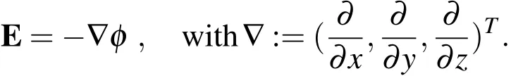
In the electrostatic case,the relation between electric fieldEand the electric potentialφis given by

Mechanical strainsSare related to the mechanical displacementsuby

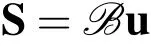
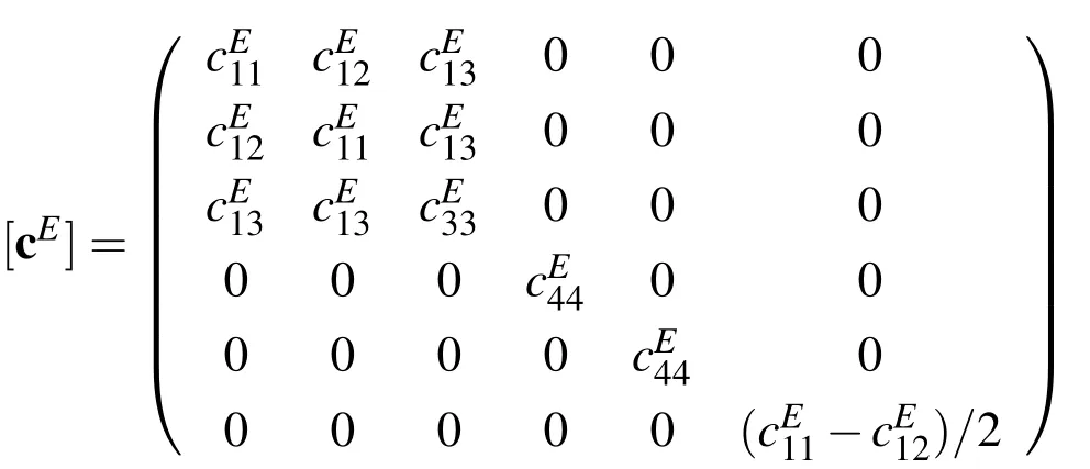
whereBis the first order differential operator relating strains and displacements.The material tensors[cE],[εS],and[e],appearing in(1),(2)are the elasticity coefficients,the dielectric constants,and the piezoelectric coupling coefficients,respectively.According to the crystal structure and polarization of the piezoelectric material,these matrices show a certain symmetry and sparsity pattern(cf.IEEEStandard(1985)).For the 6mm crystal class we have,e.g.

The mechanical behavior of piezoelectric materials is described by Newton’s law

where ρ denotes the mass density.Since piezoelectric materials are insulating,i.e.,do not contain free volume charges

Plugging the constitutive laws(1),(2)in the balance equations(5)and(6),one obtains a fully determined set of partial differential equations which are solved for the primary unknowns u and φ inside a piezoelectric domain Ω

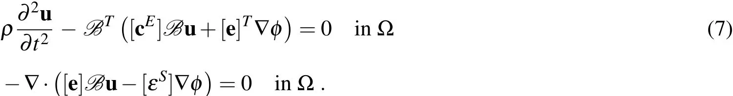
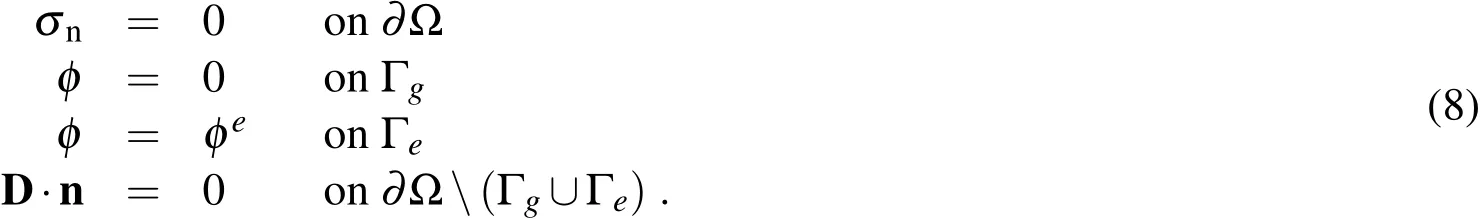
The following boundary conditions are according to the typical experimental setting of vanishing normal stresses at the boundaries,and two electrodes being applied at opposite positions Γgand Γe,one of them loaded by a prescribed electric potential φe

The application of the Fourier Transformation and Finite Element discretization to equations in(7)gives the following set of coupled algebraic equations in frequency domain,see e.g.Lerch(1990);Kaltenbacher(2004)

Herein Kuu,and Muudenote the mechanical stiffness,and mass matrix,respectively,Kφφand Kuφare the dielectric stiffness-and the piezoelectric coupling matrix.The variable ω denotes the angular frequency.The Finite Element solutions are the nodal vector of displacementsand the nodal vector of the electric potential

In order to take energy-dissipation of the material into account,complex valued material parameters are considered,which is equivalent to a velocity proportional damping in time domain.For each tensor,a constant scaling factor between the real and imaginary part is introduced assuming that an equal damping of the different entries in the material tensors is a valid approach,i.e.

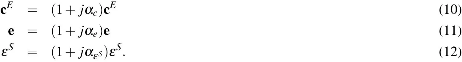
In(10),jdenotes the imaginary unit,i.e.j2=−1 in the complex number system.The eigenvalues problem in(9)is solved by the aid of the ARPACK package,see Sorensen,Lehoucq,Yang,and Maschhoff(1996),yielding the angular eigenfrequenciesω1,ω2,....The eigenfrequencies correspond to all possible mechanical eigenmodes,even the ones that cannot be excited electrically.

3 Global Sensitivity Analysis

Sensitivity analyses can be conducted in different ways.The most simple approach and mathematically motivated by the definition of a sensitivity in calculus is to compute partial derivatives.This strategy is justified for a first understanding of the problem,however,one needs to be aware that it is just alocalmeasure as it computes a parameter’s sensitivity when the values of all other parameters are fixed,i.e.assumed to be known exactly.The parameter’s sensitivity however might change drastically when the other parameters in the model contain different values.This can be exemplified regarding the sensitivity of the mechanical deflection with respect to an infinitesimal change of the mechanical damping parameter.If we are away of resonance,no significant influence will be seen.However,a change of stiffness properties may shift the resonance’s positions and the damping parameter might become visibly influential as it is now mainly responsible for the magnitude of the deflection in resonance.

Due to these interrelations,we considerglobalmeasures,where all parameters are varied while determining the sensitivity of a parameter of interest.Those methods where firstly introduced in 1973 by Cukier et.al.Cukier,Fortuin,Shuler,Petschek,and Schaibly(59)and were extended by Homma,Imam,Sobol and Saltelli,Homma and Saltelli(1996);Sobol(1990);Saltelli,Tarantola,and Chan(1999)and applied in various models in economy,engineering and science,see e.g.Sin,Gernaey,Neumann,Loosdrecht,and Gujer(2009);Keitel,Karaki,Lahmer,Nikulla,and Zabel(2011);Kami´nski and Lauke(2013).According to our knowledge,global variance-based sensitivity measures have not been applied to any qualitative assessment of models for smart materials,like piezoelectric ones.Let us assume,that in the followingFis the forward operator of our model

which maps thenmodel input parametersp1,...,pnto the model outputy=F(p1,...,pn).WithXandY,we denote the finite-dimensional parameter and measurement spaces.WithE(y)andV(y),we denote the mean and the variance of the model’s response,respectively,and byE(pi)andV(pi)fori=1,...,nthe mean and variances of the parameters.

3.1 Variance-based Sensitivity Measures

In this context,all parameters are assumed to be uncertain,i.e.they are allowed to vary according to an assumed probability distribution.Now the question arises,what happens to the variance of the model’s response,if we were able to know one parameter precisely,i.e.

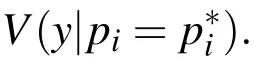
The above is the variance ofyunder the condition thatpiis known to have exactly the value.As the true value ofpicannot be assumed to be not known precisely,the mean of the conditional variance is further regarded.This measures the expected amount by which the uncertainty inyis reduced if we were able to determinepiprecisely on average.By this,the dependence of the measure onp∗iis removed.Now

is on average the expected amount of variance which is removed if we were able to knowpiprecisely.According to the decomposition of variance(law of total variance)

either a large value ofVpi(Ep～i(y|pi))or a small valueEpi(Vp～i(y|pi))implies thatpiis an important(sensitive)parameter.Normalization gives finally the definition of a first order sensitivity index

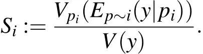
The index Siis therefore a measure of the exclusive influence of the input parameter pi.If the sum of all Siis close to one,the model is additive with respect to its variances and no remarkable interactions between the parameters seem to exist.

However,for the piezoelectric equations it is not fully understood to which extent choices of single parameters may influence each other so that higher order sensitivity measures should be evaluated in addition.The term

gives now the expected amount of variance which remains if we were able to know all parameters except piprecisely,i.e.piis allowed to vary over its uncertainty range while all other parameters are kept fixed.After normalization and applying(15)the total effects sensitivity measure is de fined as

see Sobol(1990);Homma and Saltelli(1996).The total effect index STiincludes both,the in fluence of the first order effects and all higher order(interaction)effects.Consequently,

If both sums are almost equal,then all input parameters seem to be independent.The quantities 1−∑Sior∑STi−1 are measures of the degree of interactions,which is in particular a valuable hint concerning the unique identifiability of the parameters in the associated inverse problem of parameter identification.

3.2 Computational Aspects

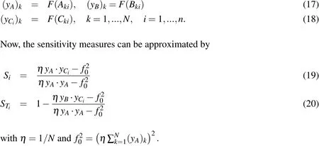
A brute force Monte-Carlo-based computation of the variance of the mean or vice versa would actually require N×N evaluations of the piezoelectric problem under investigation,where N denotes the number of samples in a Monte Carlo type simulation.Therefore,for the computation of the senstivity indices we follow the strategy poposed in Saltelli,Ratto,Andres,Campolongo,Cariboni,Gatelli,M.,and Tarantola(2008)going back to earlier approaches by Sobol(1990)and Homma and Saltelli(1996).Our implementation is based on a Latin-Hypercube Sampling strategy with which two matrices A and B of dimensions N×n are filled with random entries.The samples are generated according the assumed probability distribution of the single model parameters.The number of samples N is required to be chosen sufficiently high in order to remove any statistical uncertainty from the results.

Further matricesCi,i=1,...,nare set up then,which are equal toAexcept theith column,which is taken fromB.Now the model output,i.e.the Finite Element solution of the piezoelectric problem is computed for all rows inA,BandCiyielding 2+nvectors of lengthN.The entries are given by solving

Where as the first order sensitivity indices might rather be used in the context of research prioritization(which parameters need a more careful investigation/identification),the total order sensitivity indices provide information to which extent models can be simplified as it may be shown that some parameters are completely non-in fluential.

The random input parameters are in all cases assumed to be normally distributed and are generated using a Latin Hypercube sampling strategy,see e.g.Iman and Conover(1980).

The Finite Element simulations have been conducted with the noncommercial toolCFS++Kaltenbacher(2010)with the calculation timetFfor one model outputy=F(p1,...,pn).Pre-and post-processing is performed with MATLAB®(The MathWorks,Inc.).The effort to compute(19)and(20)is of orderO(N(n+2)).By using theParallel Computing Toolboxof MATLAB®and an appropriate computer with minimumn+2 CPU’s the computation time reduces toN·tF.

3.3 Alternative Strategies to Assess Sensitivities

Variance-based sensitivity measures provide global information,however,under sometimes prohibitive high computational costs.We therefore present two alternatives that approximate the information obtained from the variance-based sensitivity analysis.The first one measures simply correlations between input and output signals;the second alternative discusses the use of variance-based methods on surrogate models.

3.3.1 Correlation-Based Sensitivity Analysis

To anticipate,the numerical results show a rather linear relation between the system responses and uncertainties in the input parameters.Therefore,working with weighted linear correlation coefficients may give good approximations of the sensitivity indices.However,as the weighted correlation coefficients are based on Pearson’s definition of correlation,they only measure primary effects and no interactions,thus they are of the same quality as the first order effects.Correlation coefficients are de fined as

withµpi,µybeing the mean values of the model’s input and output quantities andσpi,σyare the standard deviations ofpiandy.A weighted sensitivity index based on linear correlation can now be de fined as

Besides their cheaper computation correlation coefficients provide the additional advantage that the sign of correlation(positive/negative)can be retrieved.

3.3.2 Sensitivity Analysis on Surrogate Models

As high numbers of samples are generally required to approximate the conditional variances sufficiently precise,uncertainty analysis based on response surfaces is proposed by several authors,see e.g.for the analysis of other engineering problems Marrel,Iooss,Veiga,and Ribatet(2012);Karaki(2012).Here,the true model is approximated by a response surface,also called a meta-model,which allows the main functional dependencies of the model output from model input to be represented.For rather smooth model responses,multivariate polynomial regression is generally a good choice.Any polynomial regression for models withninput parameters requires the definition of an appropriate basis,e.g.with terms of linear and quadratic order

Higher order terms could be included in this basis,however,then the problem of over fitting could become severe.According to the law of parsimony,often less complex approaches are preferable.The total number of entries in the basis is denoted bym.

The regression model is given now by

for which the regression parametersneed to be estimated.This is generally done by minimizing all residuals,i.e.the difference between the regression model and the true model’s response for every sample pointj=1,...,Nse.One method to do so is the ordinary least-squares minimization(sum of squared errors),i.e.

Minimization of this terms leads to a set of normal equations from which the coefficients can be retrieved as follows

where all regression coefficients are stored in the vector

The matrix X is the so-called Vandermonde matrix whose columns are composed by thembasis entries(see e.g.the basis in(23))which vary for every sample over theNserows,for details see,e.g.,Forrester,Sobester,and Keane(2008),Chapter 2.As long as all regression variables are linearly independent this is a well posed problem.In some contexts,a regularized version of the least squares solution could reduce the risk of non-invertability of the matrix(X┬X).Applying Tikhonov regularization one adds a constraint in the form of a penalty term to the minimization problem(24)so that the regression coefficientswill not exceed a given value.Equivalently,one may solve an unconstrained minimization problem of the sum of least-squares approach with a penalty of the formαreg‖β‖2added to the diagonal entries of(X┬X),whereαreg＞0 is a regularizing constant.In a Bayesian setting,this strategy is equal to de fining a zero-mean normally distributed prior on the parameter vector.

The so called coefficient of determinationR2

measures how well the regression model fits to the true model since it relates the explained variance(variance of the model’s predictions)

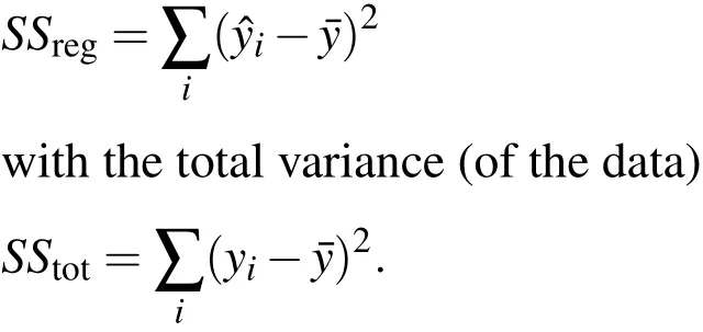
Table 1:Assumed mean values for the parameters of a Pz27 ceramicin N/m2;in As/Vm;exyin As/m2;density ρ in kg/m3).

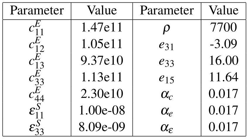
Table 1:Assumed mean values for the parameters of a Pz27 ceramicin N/m2;in As/Vm;exyin As/m2;density ρ in kg/m3).

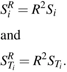
Hereyiare the model outputs,is the approximated output andis the mean value of the model output evaluated.Values ofR2close to one(at least＞0.8)are required for an acceptable approximation of the true model by the regression model.Sensitivity measures which are computed on such response surfaces need to be reduced by the factorR2as some behavior of the true model might remain unexplained,i.e.

Certainly,there are many more issues to discuss when applying regression models(reduced accuracy,over- fitting,confidence,local/global regressions,...),which however,are beyond the scope of this paper and we refer to Armstrong(2012);Cumming(2012)for further reading on these issues.

4 Results

The uncertainty analysis is conducted for two different piezoelectric problems,namely the computation of the electrical impedance of a piezoelectric disc and the computation of displacements of the tip of a piezoelectric unimorph actuator.

4.1 Electrical impedance-eigenvalue problem

Figure 1:Electrical impedance curve of a piecoelectric disc with diameter D=25mm and height h=2mm computed with the parameters as given in Table 4.1.The radial(left box)and thickness(right)resonance of the disc are visualized and can be found at～80kHz and～1MHz,respectively.

The fastest way to compute resonant frequencies is to solve the eigenvalue problem.By doing so,one obtains a list of eigenfrequencies with the corresponding eigenvectors.This list contains all mechanical eigenfrequencies of the given model,even the ones that cannot be electrically excited with the potential Φ de fined by the electrodes and the applied voltageU(see Fig.1).The major problem for this approach is the identification of the eigenfreqency that belongs to the sought-after resonance.An analysis of the eigenfrequencies and the corresponding eigenvectors shows,that every electrically excitable resonance leads to very low values of the impedance in the associated eigenvector.Since the radial resonance is the first one that can be excited electrically,it can be easily found by means of this impedance value.The frequency range around the thickness resonance also contains higher order radial modes that do not allow for a unique identifiability of the thickness resonance by means of an eigenfrequency analysis.

The second column in Table 4.1 lists the first and total order sensitivity indices with respect to the location of the radial resonance for selected parameters.The selection of the parameter is motivated by a previous parameter study Rupitsch,Sutor,Ilg,and Lerch(2010).As material a Pz27 ceramic from FERROPERM was chosen with assumed material mean-values according to Table 4.1.A check of statistical convergence revealed that after computing 100000 samples a good approximation of the sensitivity indices could be achieved.From this calculations(see Tab.4.1),we can draw directly following conclusions

·For the location of the radial resonator’s resonance,only the entries in thestiffness tensor show a significant sensitivity,especially

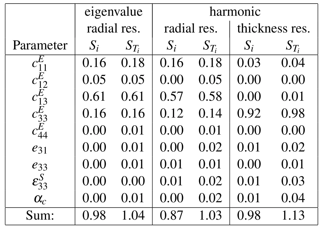
Table 2:Sensitivity indices for the resonance frequencies of a radial resonator.

·The decomposition of the system’s variance is nearly linear.98%of the uncertainty can be explained by primary effects and roughly 4%are due to interaction effects between certain variables.

·The interaction is mainly affecting the parameter

4.2 Electrical impedance-harmonic analysis

In the following,the sensitivity analysis was applied to a harmonic analysis of a piezoelectric disc where both the fundamental radial and the thickness resonance are investigated.Simulations have been conducted for 400 linearly distributed frequencies around the resonances.In detail,the frequency ranges 70–90 kHz and 850–1050 kHz are considered and the resonances are given by searching for the minimum impedance within these ranges.Table 4.1 shows that the harmonic analysis results in the same sensitivities as w.r.t.the solution of the eigenvalue problem(compare columns two and three).The calculated sensitivity indices for the thickness resonance allow for the following conclusion:

·For the location of the thickness resonance onlyshows a significant sensitivity.

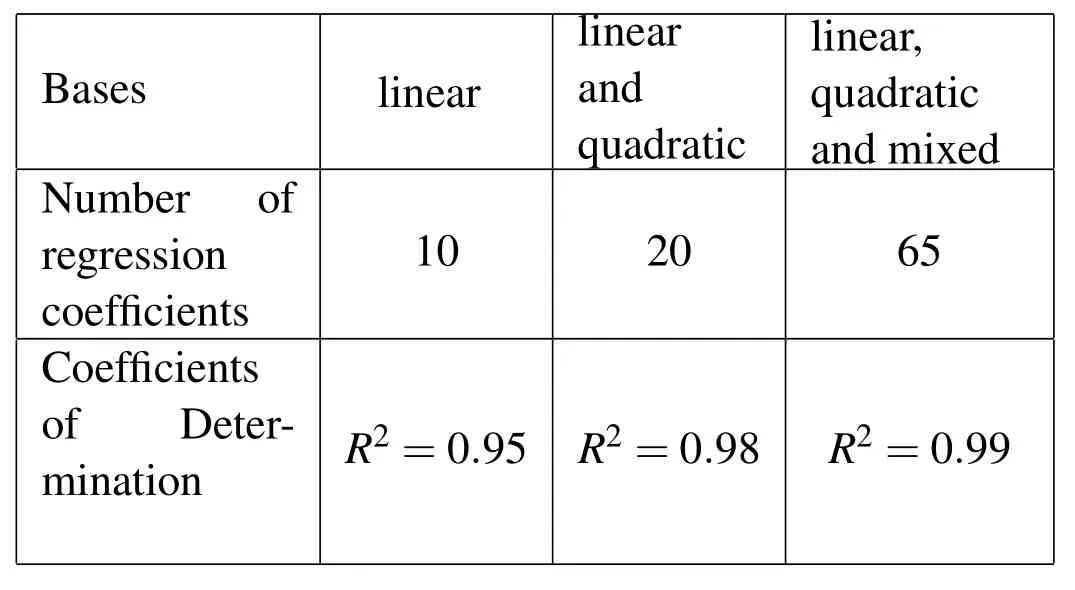
Table 3:Coefficients of Determination Using different Bases for the Regression Model.

·The decomposition of the system’s variance is also approximately linear.98%of the uncertainty can be explained by primary effects and roughly 13%are due to interaction effects between certain variables.

·The interaction is mainly affecting the parameters

4.3 Piezoelectric unimorph-static analysis-UA based on response surfaces

The strategy of applying sensitivity measures on regression models is now applied to a piezoelectric unimorph modeled in 3D as it is assumed to be„too costly"for an analsyis directly on the model.The unimorph consists of two plates,a piezoelectric ceramic,Pz27,and copper sheet,which are glued together.The piezoelectric layer is polarized in the third dimension(z),the electrodes are always inx−yplane,see Figure 2.For the copper,a Young’s modulus of 9.6e+10Paand a Poisson ratio of 0.3 are assumed.

Different bases for setting up a polynomial regression model have been tested leading to coefficients of determination as given in Table 4.3,which allows for a very good approximation of the true model behavior.For setting up the regression models,500 samples have been generated with a coefficient of variation of 5%.The sensitivity measures computed on the regression model with linear,quadratic and mixed quadratic terms are reported in the Tables 4.3 and 4.3.For the generation of the random input parameters,a coefficient of variation of 2%was assumed and 200000 samples have been evaluated on the regression model.The values in Table 4.3 belong to a model where theZdirection corresponds with the 3 direction of the material.In Table 4.3 a reorientation of the material is assumed so that theZdirection of the model is now the 1 direction of the material.As for setting up the regression models,already a series of model responses needs to be computed,a sensitivity analysis based on correlation can be conducted additionally,where the results are reported in Tables 4.3 and 4.3 in the third last column.

Figure 2:Displacement field and electric potential of a piezoelectric unimorph polarized in z-direction.The unimorph is mechanically clamped at the left-hand side(y=0).

The findings have shown that sensitivity analysis on regression models give quite accurate approximations of the real sensitivities,however,with a significantly reduced computational time.The analysis of the unimorph with a reoriented material serves mainly academic considerations as it shows sensitivities of the parameters for less common models where experiences about the main input parameters are less available.As we see,indices based on correlation give a fair approximation to the variance-based indices and may also be used for the purpose of factor prioritization.

Remark:By comparing the changes in the results while evaluating new samples,one can de fine a stopping criterion.With this criterion an upper limit of samples can be determined.See Figure 3 for the convergence of the sum of all sensitivity measures for the unimorph example assuming uniformly distributed input parameters.As the sensitivity indices are approximated by stochastic sampling schemes,the results are only to be regarded as estimates of the true values.The accuracy of these estimates depends mainly on the number of simulation runs,the assumed scatter in the input parameters and the number of parameters in the model.A too small number of simulations or poorly chosen samples may give inaccurate results.

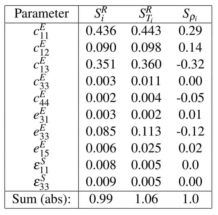
Table 4:Sensitivity Indices of a 3 D Model unimorph for the displacements in Z(3)direction under static analysis.Z-Polarization on a response surface with mixed quadratic terms.

Table 5:Sensitivity Indices of a 3 D Model unimorph for the displacements in Z(1)direction under static analysis.Z-Polarization on a response surface with mixed quadratic terms.

Figure 3:Convergence of first and total order sensitivity indices,logarithmic scale.

These are visible,e.g.when sensitivity indices close to zero have a negative sign or when someSivalues are larger than theSTivalues.If these effects are rather visible,it is recommended to repeat the sampling with a higher number of samples.Results are only reliably with respect to the second position after the decimal point.Repeated analyses and averaging would yield more robust results.

5 Conclusion and Outlook

From the numerical results one can draw the conclusion that for the applications discussed here,the variance in the responses of piezoelectric models might be separated in an almost additive manner according to the variances of the single input parameters.The relatively small differences in the values of first-order and totalorder sensitivity measures allow such conclusions.However,the result might be different when looking at further objectives,e.g.the quality factor or the emitted waves of a piezoelectric ultrasound generator.Variance-based methods are proven to be a valuable tool in analysing and studying piezoelectric models of moderate complexity.For larger models,the high computational costs may limit the applicability of the proposed methods.In those cases,indices computed with regression models or correlation-based measures have been shown to be an acceptable approximation.In order to obtain more precise statistical information about the model input parameter’s,a parameter estimation in the framework of Bayesian model updating should be conducted.The result of those inversions is a so calleda posterioriprobability from which all statistical moments can be retrieved.Those results will mainly be dependent on the number of measurements and the measurements’noise.

Acknowledgement:The second and third author gratefully acknowledges the support of the German Research Foundation(DFG)in context of the Collaborative Research Centre/Transregio 39 PT-PIESA,subproject C6.

The authors additionally want to thank the reviewers and Dr.Holger Keitel,Dr.Stephan Rupitsch and Peter Olney for their careful reading of the manuscript.

Alwan,A.;Aluru,N.(2011):Uncertainty quantification of MEMS using a datadependent adaptive stochastic collocation method.Comput.Methods Appl.Mech.Engrg,vol.200,pp.3169–3182.

Armstrong,J.S.(2012):Illusions in regression analysis.International Journal of Forecasting(forthcoming).

Cukier,R.I.;Fortuin,C.M.;Shuler,K.;Petschek,A.;Schaibly,J.(59):Study of the sensitivity of coupled reaction systems to uncertainties in rate coefficients.Theory.J.Chem.Phys,vol.1973.

Cumming,G.(2012):Understanding The New Statistics:Effect Sizes,Con fidence Intervals,and Meta-Analysis.Routledge,New York.

Du,X.-H.;Wang,Q.-M.;Uchino,K.(2004):An accurate method for the determination of complex coefficients of single crystal piezoelectric resonators I:Theory.IEEEUFFC,vol.51,pp.227–235.

Dziatkiewicz,G.;Fedelinski,P.(2007):Dynamic analysis of piezoelectric structures by the dual reciprocity boundary element method.Computer Modeling in Engineering&Sciences,vol.17,no.1,pp.35–46.

Forrester,A.;Sobester,A.;Keane,A.(2008):Engineering Design via Surrogate Modelling.John Wiley and Sons Ltd.

Homma,T.;Saltelli,A.(1996):Important measures in global sensitivity analysis of nonlinear models.Reliability Engineering And System Safety,vol.52,pp.1–17.

IEEEStandard(1985):IEEE Standard on Piezoelectricity,1985.IEEE/ANSI.

Iman,R.;Conover,W.(1980): Small sample sensitivity analysis techniques for computer models with an application to risk assessment.Communications in Statistics,vol.17,no.9,pp.1749–1842.

Jonsson,U.;Andersson,B.;Lindahl,O.(2013):A FEM-based method using harmonic overtones to determine the effective elastic,dielectric,and piezoelectric parameters offreely vibrating thick piezoelectric disks.IEEE Transactions on Ultrasoncis,Ferroelectrics and Frequency Control,vol.60,no.1,pp.243–235.

Kaltenbacher,B.;Lahmer,T.;Mohr,M.(2006):PDE based determination of piezoelectric material tensors.European Journal of Applied Mathematics.

Kaltenbacher,M.(2004):Numerical Simulation of Mechatronic Sensors and Actuators.Springer Berlin-Heidelberg-New York.ISBN:3-540-20458-X.

Kaltenbacher,M.(2010):Advanced simulation tool for the design of sensors and actuators.Proc.Eurosensors XXIV,vol.5,pp.597–600.

Kami´nski,M.;Lauke,B.(2013):Parameter sensitivity and probabilistic analysis of the elastic homogenized properties for rubber filled polymers.Computer Modeling in Engineering&Sciences,vol.93,no.6,pp.411–440.

Karaki,G.(2012):Assessment of coupled models of bridges considering timedependent vehicular loading.PhD thesis,Bauhaus University Weimar,Germany,DFG-Research Training Group 1462 „Modelquality”,2012.

Keitel,H.;Karaki,G.;Lahmer,T.;Nikulla,S.;Zabel,V.(2011):Evaluation of coupled partial models in structural engineering using graph theory and sensitivity analyses.Engineering Structures,vol.33,pp.3726–3736.

Kwok,K.W.;Chan,H.L.W.;Choy,C.L.(1997):Evaluation of the material parameters of piezoelectric materials by various methods.IEEEUFFC,vol.44,no.4,pp.733–742.

Lahmer,T.(2009): Modified landweber iterations in a multilevel algorithm applied to inverse problems in piezoelectricity.Journal of Inverse and Ill-Posed Problems,vol.17,no.1.

Lahmer,T.;Kaltenbacher,B.;Schulz,V.(2008): Optimal experiment design for piezoelectric material tensor identification.Inverse Problems in Science and Engineering,vol.6,pp.369–387.

Lahmer,T.;Kaltenbacher,M.;Kaltenbacher,B.;Leder,E.;Lerch,R.(2008):FEM-based determination of real and complex elastic,dielectric and piezoelectric moduli in piezoceramic materials.IEEE Transactions on Ultrasonics,Ferroelectrics,and Frequency Control,vol.55,no.2,pp.465–475.

Lerch,R.(1990): Simulation of piezoelectric devices by two-and threedimensional finite elements.IIEEE Transactions on UFFC,vol.37,no.3,pp.233–247.ISSN 0885-3010.

Marrel,A.;Iooss,B.;Veiga,S.;Ribatet,M.(2012):Global sensitivity analysis of stochastic computer models with joint metamodels.Statistics and Computing,vol.22,no.3,pp.833–847.

Most,T.(2011):Assessment of structural simulation models by estimating uncertainties due to model selection and model simplification.Computers&Structures,vol.89,no.17-18,pp.1664–1672.

Olyaie,M.S.;Razfar,M.R.;Kansa,E.J.(2011): Reliability based topology optimization of a linear piezoelectric micromotor using the cell-based smoothed finite element method.Computer Modeling in Engineering&Sciences,vol.75,no.1,pp.43–88.

Olyaie,M.S.;Razfar,M.R.;Wang,S.;Kansa,E.J.(2011): Dynamic analysis of piezoelectric structures by the dual reciprocity boundary element method.Computer Modeling in Engineering&Sciences,vol.82,no.1,pp.55–82.

Poteralskia,A.;Szczepanika,M.;Dziatkiewicza,G.;W.,K.;Burczyn´skiab,T.(2011):Immune identification of piezoelectric material constants using BEM.Inverse Problems in Science and Engineering,vol.19,no.1,pp.103–116.

Rupitsch,S.;Sutor,A.;Ilg,J.;Lerch,R.(2010): Identification procedure for real and imaginary material parameters of piezoceramic materials.Ultrasonics Symposium(IUS),2010 IEEE,pp.1214–1217.

Rupitsch,S.;Wolf,F.;Sutor,A.;Lerch,R.(2012): Reliable modeling of piezoceramic materials utilized in sensors and actuators.Acta Mechanica,pp.1–13.10.1007/s00707-012-0639-7.

Rupitsch,S.J.;Lerch,R.(2009): Inverse method to estimate material parameters for piezoceramic disc actuators.Applied Physics A:Materials Science and Processin,vol.97,no.4,pp.735–740.

Rus,G.;Palma,R.;Pérez-Aparicio,J.L.(2011): Experimental design of dynamic model-based damage identification in piezoelectric ceramics.Mechanical Systems and Signal Processing,vol.26,pp.268–293.

Saltelli,A.;Ratto,M.;Andres,T.;Campolongo,F.;Cariboni,F.;Gatelli,D.;M.,S.;Tarantola,S.(2008):Global Sensitivity Analysis.J.Wiley&Sons.Ltd.

Saltelli,A.;Tarantola,S.;Chan,K.(1999): Quantitative model-independent method for global sensitivity analysis of model output.Technometrics,vol.41,no.1,pp.39–56.

Sherrit,S.;Wiederick,H.D.;Mukherjee,B.K.(1992): Non-iterative evaluation of the real and imaginary material monstants of piezoelectric resonators.Ferroelectrics,vol.134,pp.111–119.

Sherrit,S.;Wiederick,H.D.;Mukherjee,B.K.(1997): A complete characterization of the piezoelectric,dielectric,and elastic properties of Motorola PZT 3203 HD,including losses and dispersion.SPIE Proceedings,vol.3037-22,pp.158–169.

Sin,G.;Gernaey,K.;Neumann,M.;Loosdrecht,M.;Gujer,W.(2009):Uncertainty analysis in WWTP model applications:A critical discussion using an example from design.Water Research,vol.43,no.11,pp.2894–2906.

Sobol,I.M.(1990): Sensitivity estimates for nonlinear mathematical models.Matematicheskoe Modelirovanie,vol.2,pp.112–118.

Sorensen,D.;Lehoucq,R.;Yang,C.;Maschhoff,K.(1996):ARPACK Homepage-http://www.caam.rice.edu/software/arpack/,1996.

Zhang,X.;Xu,X.;Wang,Y.(2014): Wave propagation in piezoelectric rods with rectangular cross sections.Computer Modeling in Engineering&Sciences,vol.100,no.1,pp.1–17.

1Bauhaus University Weimar,Germany

2Friedrich-Alexander University,Erlangen-Nuremberg,Germany