Numerical study of corner separation in a linear compressor cascade using various turbulence models

Liu Yangwei,Yan Hao,Liu Yingjie,Lu Lipeng,Li Qiushi

Collaborative Innovation Center of Advanced Aero-Engine,Beihang University,Beijing 100083,China

National Key Laboratory of Science and Technology on Aero-Engine Aero-Thermodynamics,School of Energy and Power Engineering,Beihang University,Beijing 100083,China

Numerical study of corner separation in a linear compressor cascade using various turbulence models

Liu Yangwei,Yan Hao,Liu Yingjie*,Lu Lipeng,Li Qiushi

Collaborative Innovation Center of Advanced Aero-Engine,Beihang University,Beijing 100083,China

National Key Laboratory of Science and Technology on Aero-Engine Aero-Thermodynamics,School of Energy and Power Engineering,Beihang University,Beijing 100083,China

Three-dimensional corner separation is a common phenomenon that significantly affects compressor performance.Turbulence model is still a weakness for RANS method on predicting corner separation flow accurately.In the present study,numerical study of corner separation in a linear highly loaded prescribed velocity distribution (PVD)compressor cascade has been investigated using seven frequently used turbulence models.The seven turbulence models include Spalart–Allmaras model,standard k–ε model,realizable k–ε model,standard k–ω model,shear stress transport k–ω model,v2–f model and Reynolds stress model.The results of these turbulence models have been compared and analyzed in detail with available experimental data.It is found the standard k–ε model,realizable k–ε model,v2–f model and Reynolds stress model can provide reasonable results for predicting three dimensional corner separation in the compressor cascade.The Spalart–Allmaras model,standard k–ω model and shear stress transport k–ω model overestimate corner separation region at incidence of 0°.The turbulence characteristics are discussed and turbulence anisotropy is observed to be stronger in the corner separating region.

1.Introduction

Three-dimensional(3D)corner separation in compressor cascade has been considered as an inherent flow phenomenon in compressor cascade.1It has great impact on compressor performance,such as higher total pressure loss,static pressure rising limitation,compressor efficiency reduction,passage blockage,and stall and surge especially for highly loaded compressor.2Many efforts have been made on studying the corner separation by experimental investigations3–5and numerical simulations6,7under various conditions over the past few years.Several flow controlling techniques have been utilized to improve compressor performance recently.8–11The basic structures and characteristics of 3D corner separation are well-summarized12,thus their primary effects on compressor performance have been considered in designing process and have improved compressor performance greatly.In compressor routine design,the corner separation should be accurately predicted by employing computational fluid dynamics(CFD).

The CFD technique has been widely used and has played an increasingly important role in the aerodynamic design routine of compressor.The Reynolds-averaged Navier–Stokes equations(RANS)method is still the most widely used approach in industrial CFD due to the computational cost and design schedule,though direct numerical simulation(DNS),large eddy simulation(LES)and hybrid LES/RANS(such as detached eddy simulation(DES)13,scale adaptive simulation(SAS)14)have been used to investigate flow mechanisms in relative low Reynolds number with simple boundary.15–18According to Spalart19,20,while it has been assumed that limitless increases in computing power will someday remove the need for turbulence modeling,the estimates for this milestone have been close to the year 2080,which is a long time away.

Turbulence model is one of the key elements and is currently a weakness for RANS approach.Far less precision has been achieved in turbulence modeling since a mathematical model has been created to approximate the complicated physical behavior of turbulent flows.It is generally acknowledged not any turbulence model is suitable for all kinds of complex flow problems.21Hence,the performance of various widely used turbulence models should be assessed for a certain kind flow and then be improved.22–27Then we could build up the scope of application for various turbulence models.

The next high-power-density generation aeroengines must be supported by more advanced compressors in the future and this requires that the RANS method applied in designing process can predict main flow structures in compressor cascade to decrease designing risk as much as possible.It is very practical and critical to simulate the corner separation accurately by using RANS approach.However,it is a big challenge for RANS method to precisely predict such complicated turbulent flow field,because the 3D corner separation contains complex vortices and large separation in cascade corner region.28

In this paper,seven turbulence models which are frequently applied in engineering have been used in the detailed numerical investigations using software FLUENT for a linear highly loaded compressor cascade experimentally studied by Gbadebo et al.29In order to minimize grid impacts on numerical results,great efforts for the grid generation have been made till grid independence was obtained.The numerical results of seven turbulence models have been compared with experimental data carefully.The turbulence characteristics are discussed for analyzing the mechanisms for discrepancies.This study provides a worthy reference for using turbulence models properly and helps designers understand numerical results further.It provides valuable reference on modifying turbulence models for 3D corner separation.

2.Numerical method

In this study,the same numerical platform and grid have been used to minimize other factors'effects on numerical results

when assessing different turbulence models.The commercial flow solver package FLUENT30is applied to conduct numerical simulation in the cascade.

2.1.Governing equations and turbulence models

The governing equations of steady RANS method for incompressible fluid field are as follows:

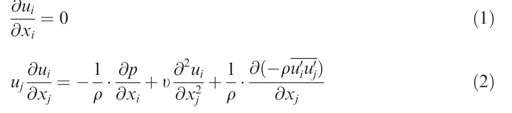
where ρ is density of the fluid,p is pressure of the fluid,uiis a mean component of velocity in the direction xi.υ is kinematic viscosity.The additional fluctuation quantitiesare unknown Reynolds-stress tensors,whilerepresents the velocity fluctuation in i-direction,the bar above represents the time-averaged result of the invariant.

In the momentum equation,the Reynolds stress tensors

are unknown which makes this equation unclosed.The Reynolds stress tensors are modeled by turbulence model.Turbulence models utilized in the study except for the Reynolds stress model are based on the Boussinesq hypothesis,which is expressed as follows:

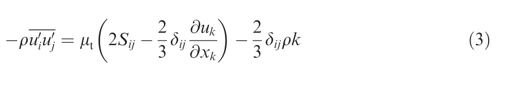
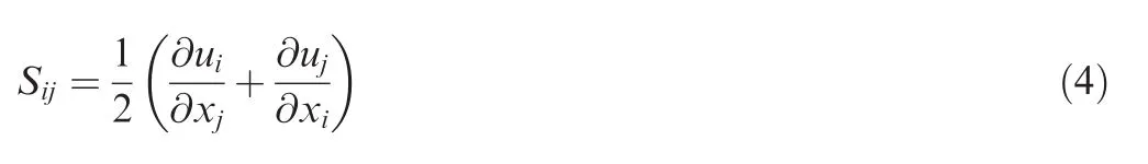
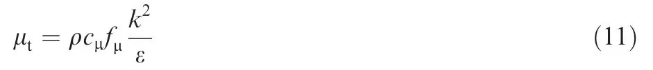
where μtis turbulent viscosity,δijis Kronecker delta function(δij=1 if i=j and δij=0 if i≠ j),k is the turbulent kinetic energy.The repeated index implies summation from 1 to 3.Sijis the mean strain-rate tensor which is calculated as

Turbulent viscosity μtare modeled by various turbulence models.The transport equations are different from one turbulence model to another,so the turbulence viscosity is quite different which leads to discrepancies on the results of complicated turbulent flow field.

(1)Spalart–Allmaras model(SA)As a simple one-equation model,the SA model solves a transport equation for the kinematic eddy viscosity.It has been proposed and developed by Spalart and Allmaras31,32since 1992.The transportation equation of this model in FLUENT is as follows:

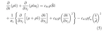
The turbulent viscosity is computed as

and

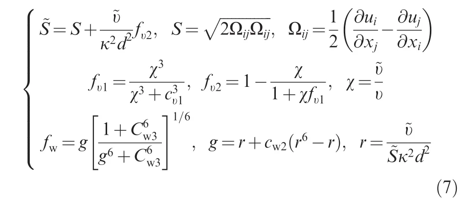
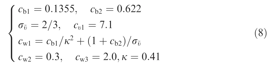
where t denotes time,~υ is modified eddy viscosity,which is the working variable calculated in Eq.(5),μ is the molecular viscosity,υ is kinematic eddy viscosity and d denotes the distance from the field point to the nearest wall.cb1,cb2, σ~υ,cυ1,cw1,cw2,cw3,and κ are constant coefficients.Their values are:

(2)Standard k–ε model(SKE)

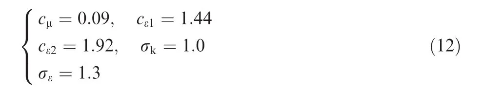
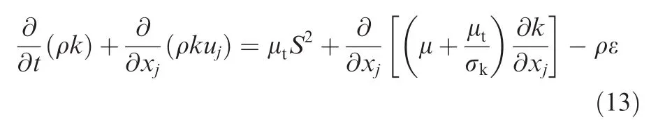
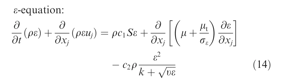
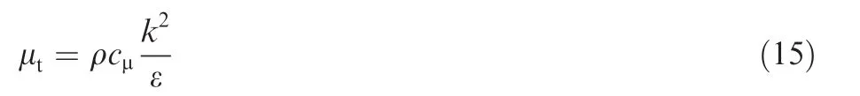
The SKE model was developed by assuming the flow is fully turbulent without consideration of molecular viscosity effects33,34.This model requires an additional model,which includes impacts of molecular viscosity for near wall regions.The transportation equations of this model in FLUENT are as follows:k-equation:

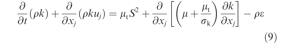
ε-equation:

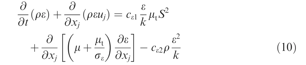
The turbulent viscosity μtis computed as

(3)Realizable k–ε model(RKE)

The RKE model has been developed from SKE and satisfies mathematical constraints on Reynolds stress.35The RKE model can provide accurate predictions on flows that involve rotation,boundary layers under strong adverse pressure gradients,separation and recirculation.The transportation equations of this model in FLUENT are as follows:k-equation:

where Sijrefers to

Eq.(4).c2=1.9The turbulent viscosity is computed as

The constants(σk,σε)have the same values as for standard k–ε model.The parameter cμcan be referred from User's Guide in FLUENT.30

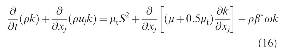
(4)Standard k–ω model(SKW)

The SKW model contains two transport equations which correspond to turbulence kinetic energy and specific dissipation rate.36The transportation equations of this model in FLUENT are as follows:k-equation:

ω-equation:

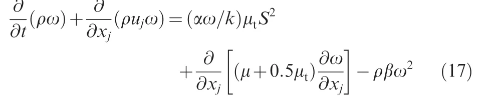
The turbulent viscosity is computed as

where ω is specific dissipation rate.The related constant parameters are:

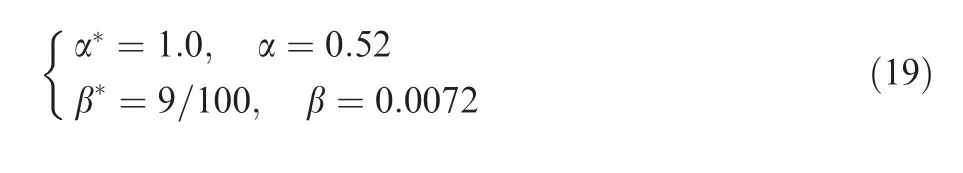
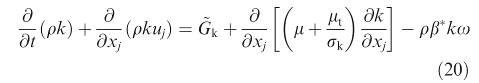
(5)Shear stress transport k–ω model(SST)

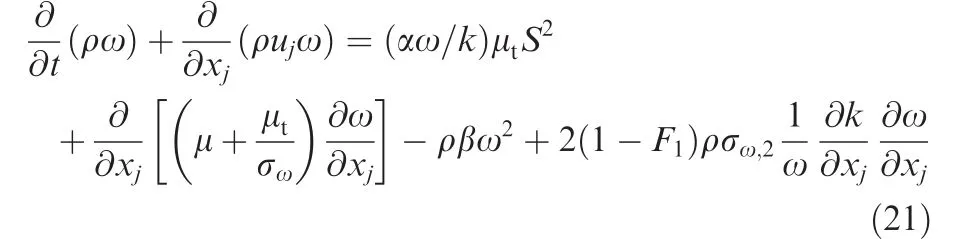
Menter37developed SST model,which calculates turbulent flow field with SKW model in the near wall region and switches to SKE model in the far field.Blending functions are used in this model.The transportation equations of this model in FLUENT are as follows:kequation:

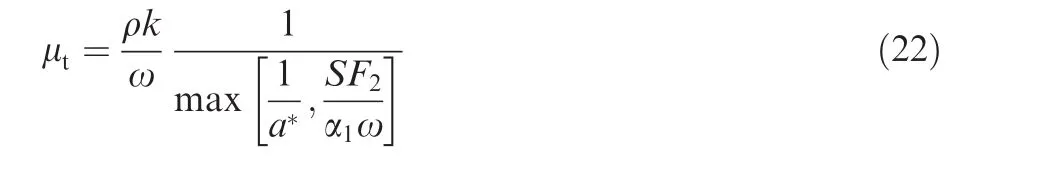
ω-equation:

The turbulent viscosity is computed as

(6)v2–f model(V2F)Durbin38proposed v2–f model which requires solutions of three transport equations and one elliptic equation.This four-equation model based on transport equations for the turbulence kinetic energy(k),dissipation rate(ε),a velocity variance scale(v2),and an elliptic relaxation function(f).The v2–f model is a low-Reynolds-number turbulence model which uses velocity scale(v2)instead of turbulent kinetic energy to evaluate turbulent viscosity.39,40The equations for turbulent kinetic energy and the dissipation rate are the same as those of the standard k–ε model,while the equations for v2andfcan be written as follows:The v2-equation:

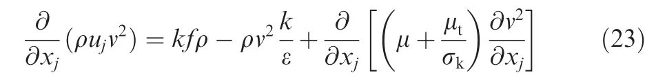
The f-equation:

where:

Here σk=1.0 cμ=0.22

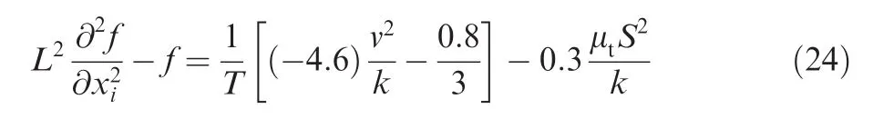
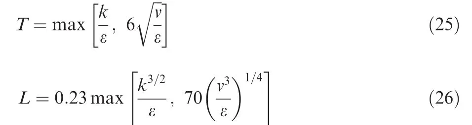
(7)Reynolds stress model(RSM)The RSM model41,42contains seven transportation equations which close RANS momentum equations by solving Reynolds stresses directly and combine with an equation for dissipation rate.The RSM is seldom selected in simulating complicated engineering applications because the robustness and computational cost of the RSM are noticeably inferior to eddy-viscosity models.43The transport equations without the effects of buoyancy are shown as

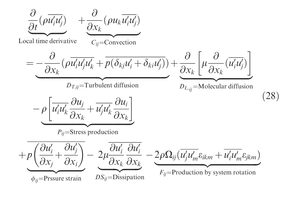
where εjkmis Levi–Civita symbol.The turbulent diffusion DT,ijis defined by using a simplified version of the generalized gradient-diffusion model,which is

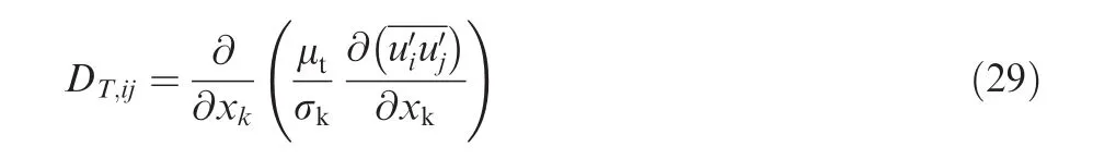
Here,σkis a constant equal to 0.82.

The pressure-strain term φijis defined as

where the slow pressure-strain term φij,1is defined as

结果如图4所示，Rh2-S诱导K562和KG1a细胞24 h后，与对照组比较，促凋亡蛋白Bax与抑凋亡蛋白Bcl-2的比值增加；周期蛋白Cyclin D1表达水平降低（P＜0.05）。说明Rh2-S可以促进K562和KG1a细胞凋亡，并有效阻滞细胞周期。

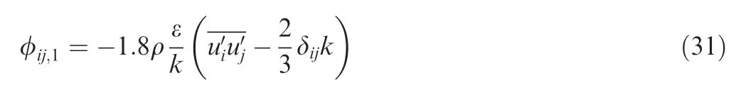
and the rapid pressure-strain term φij,2is defined as

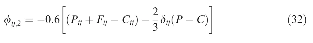
where P=0.5Pkk,C=0.5Ckk,the repeated index implies summation from 1 to 3.

The dissipation tensor DSijis defined as

The equation for dissipation rateεis the same as that of the standard k–ε model.

2.2.Linear compressor cascade

One prescribed velocity distribution(PVD)high-load linear compressor cascade,which was experimentally investigated at Cambridge University29,44–46,is used as a computational case in the current study.In our previous studies9,10,flow control and flow mechanisms for corner separation were conducted in the same cascade.The parameters of this cascade are summarized in Table 1,where c is the chord length,s is the pitchwise distance,h is the height of blade and t is the maximum blade thickness.

In this study,one-blade passage is used to conduct the numerical simulation.Two sides of the flow passage are set as periodic boundary conditions.Because of no tip clearance in the cascade,the computational domain is cut to half span and the passage top surface is set as symmetric condition in order to reduce computation quantity.

The grid topology is O4H and the point distribution is shown in Fig.1(a).Hexahedral structural meshes are generated by software NUMECA,AutoGrid5TM,as shown in Fig.1(b).The y+of first grid adjacent to the wall is approximate 1.0.Series cases with different grid numbers and grid distributions have been tested to examine the grid independence of thesolution.Finally,the case with 3 million grids is selected for the calculation and applied for different turbulence models.

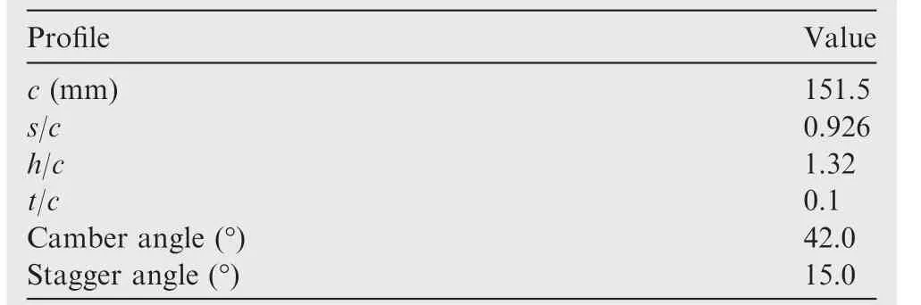
Table 1 Geometric parameters of cascade.

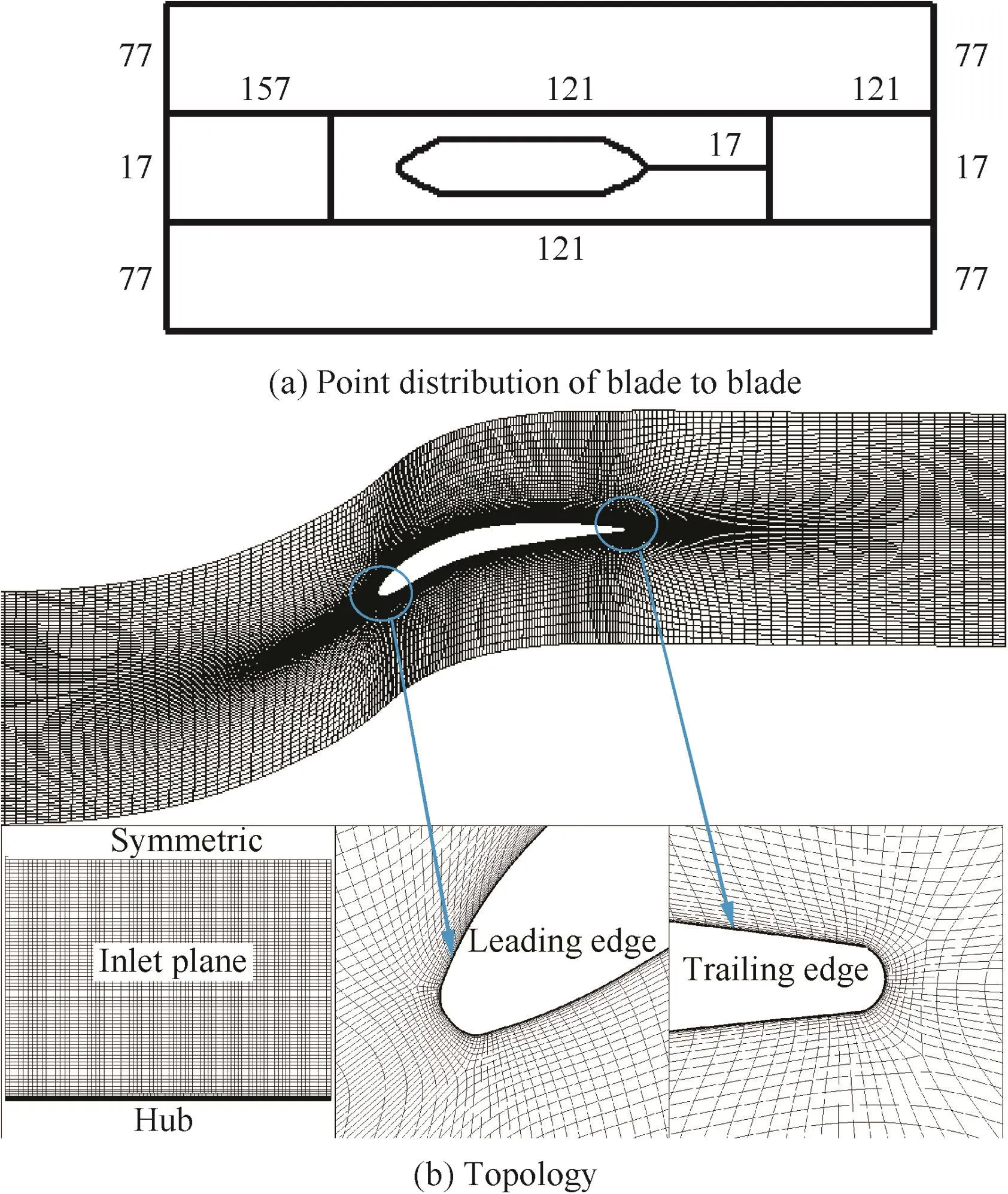
Fig.1 Grids of PVD cascade.

Enhanced wall treatment30is applied to simulating the turbulent flow for the SKE,RKE and RSM in the near-wall region.In current studies,the enhanced wall treatment can possess the accuracy of the standard two-layer model in the near-wall region because of the fine near-wall meshes used in the simulations.

2.3.Numerical scheme and boundary conditions

The second-order upwind scheme is used for the convection terms and the viscous terms of each governing equation to minimize the numerical diffusion.Other numerical schemes can be described in detail in the FLUENT User's Guide.30According to the experiment,the velocity of the main flow(U1)is 23.0 m/s,U is the local velocity at inlet.The profile of boundary layer at inlet is shown in Fig.2.The turbulent intensity is 1.5%at inlet.Moreover,all the solid walls are set as non-slip conditions.

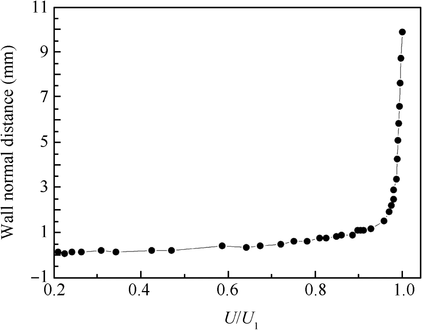
Fig.2 Velocity profile at inlet.

2.4.Definitions of flow field parameters

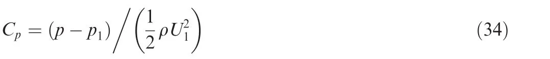
Several important performance parameters in compressor cascade are defined as follows.The static pressure coefficient is defined as

Another important parameter is total pressure loss which is defined as

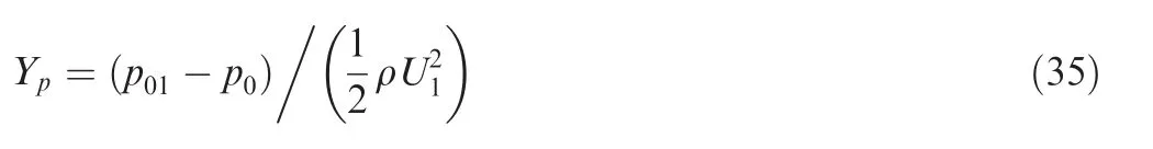
where the reference total pressure(p01)was measured in the inlet free stream with a side wall static pressure(p1)at similar location where the inlet velocity profile was measured.p0is total pressure at the local point.

The relative displacement thickness29can represent the thickness of 3D separating layer,which is defined as

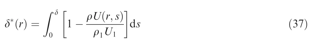
where δ is boundary layer thickness,r is radial distance,ρ1is the density at inlet.U(r,s)is the local velocity.

3.Results and discussion

3.1.Validations of different turbulence models

The streamlines on the endwall shown in Fig.3 can represent the corner separation scale in PVD cascade using different turbulence models.Compared with oil flow visualization in experiment,the corner separating scales from RSM,SKE,RKE and V2F models show good agreement with experiment and no reverse flow is observed on the endwall.The separating scales are obviously large in the results of SA,SKW and SST models and reverse flow appears on the endwall,which indicates that corner stall happens in the cascade.The low-speed area besides the rear part of blade suction surface can also reflect the corner separation scale.From the contour of velocity magnitude shown in Fig.4,the low-speed areas in RSM,SKE,RKE and V2F models are obviously smaller than the results of SA,SKW and SST models at 0°incidence.

Fig.5 shows the static pressure coefficient(Cp)at mid-span region(54%span)and hub region(89%span)using seven RANS turbulence models at incidences of-7°and 0°respectively.Fig.5(a)and(b)indicate that all turbulence models,except the SKW model,provide reasonable results at the incidence of-7°at the mid-span region and hub region respectively.Cpin the SKW model exhibits a slight discrepancy at the hub region(89%span).Given that the cascade works at the negative incidence,3D corner separation is determined to be small.In this condition,these commonly-used turbulence models can provide reasonable results.Fig.5(c)reveals that the RANS methods provide reasonable predictions at the blade mid-span region at the incidence of 0°because corner separation is small.However,the discrepancy becomes significant at the hub region.The lines of SA,SKW and SST model become flat behind 40%chord as shown in Fig.5(d),which indicates that these models predict earlier boundary separation and larger corner separation in the cascade than other models.

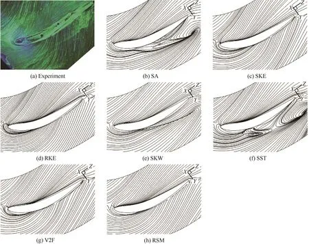
Fig.3 Streamlines on endwall at 0°incidence.

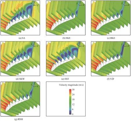
Fig.4 Contour of velocity magnitude in cascade at 0°incidence.

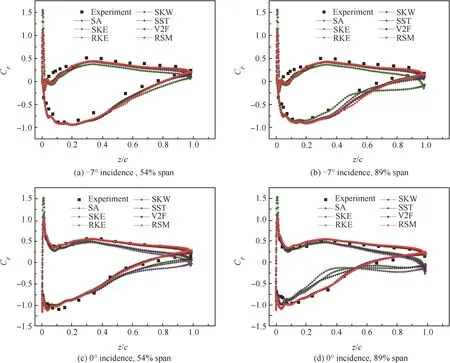
Fig.5 Static pressure coefficient on blade surface.

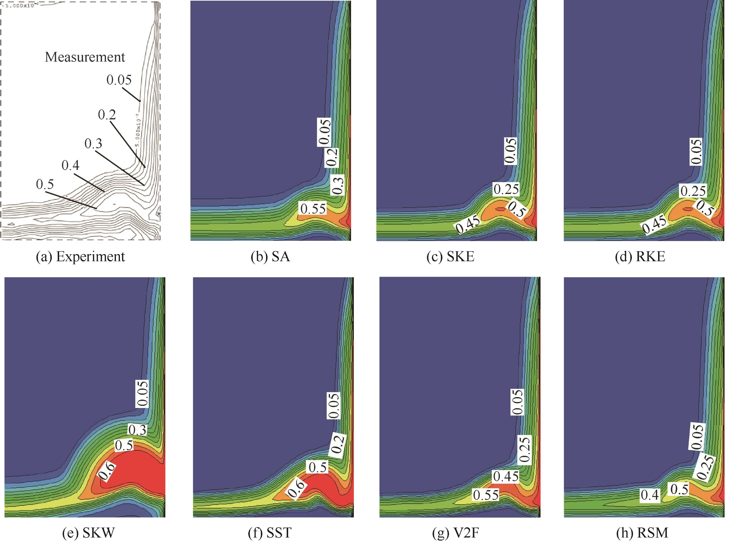
Fig.6 Contour of total pressure loss at-7°incidence.

Fig.6 illustrates total pressure loss contour coefficient at-7°incidence.The total pressure loss in corner region is high-loss area in compressor cascade,which is called''loss core areaquot;in this paper.The boundary layer thickness and the wake from the results of the seven turbulence models are not as thick as those in the experiment.The loss core areas in the results of SA,V2F,SKE,RKE,SST,and RSM models are similar to those in the experiment,whereas the loss core area in SKW model is obviously larger than the other models.This finding indicates larger corner separation in the SKW model which matches to the results of the pressure coefficient in Fig.5(b).

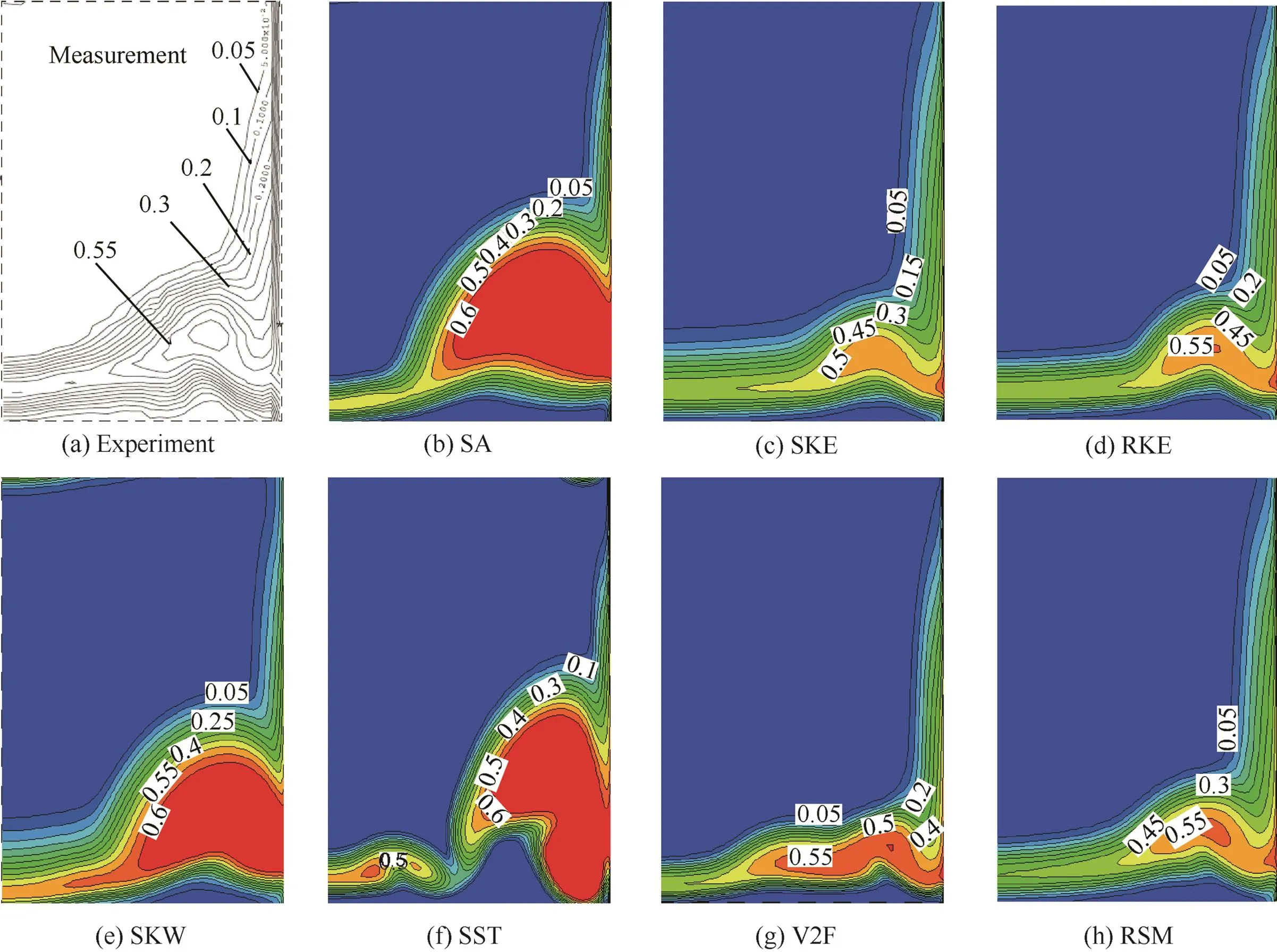
Fig.7 Contour of total pressure loss at 0°incidence.

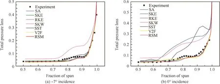
Fig.8 Pitchwise mass-averaged total pressure loss.

Fig.9 Outflow angle.

When the incidence reaches at 0°,the results of SKE,RKE,V2F and RSM agree better with measurement,while the results of SA,SKW and SST model predict unreasonably larger loss core area in the cascade from Fig.7.Relatively,the shape of corner region predicted by V2F is a little different from experiment.Fig.8(b)shows that the pitchwise mass averaged total pressure loss exhibits the same trend.The total pressure loss from SKW,SST and SA model is obviously higher than that from experiment near the endwall.

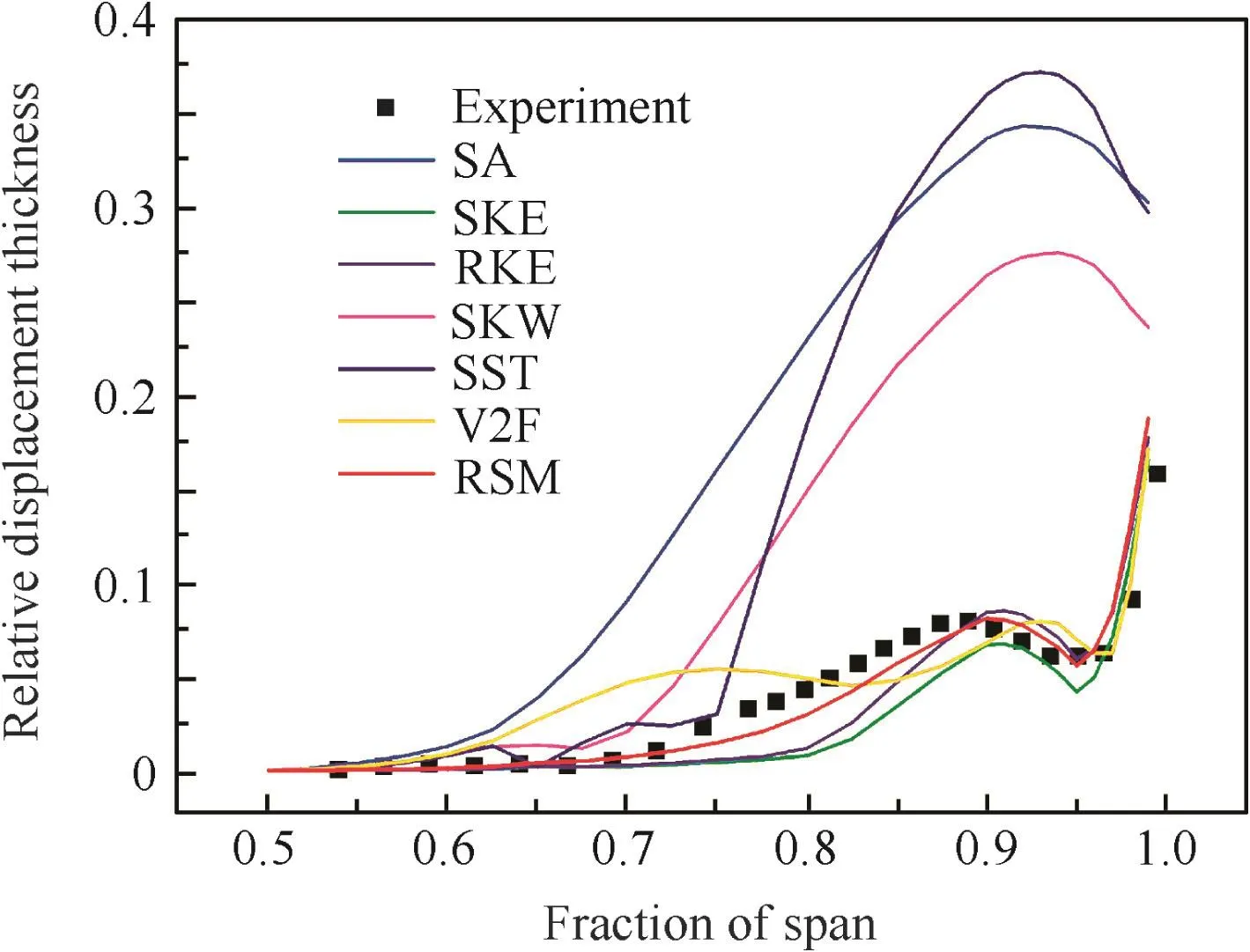
Fig.10 Relative displacement thickness at 0°incidence.

The pitchwise mass-averaged total pressure losses at-7°and 0°incidences are shown in Fig.8.When the cascade works at-7°incidence,the corner separation region is not obvious and these turbulence models except for the SKW model can provide reasonable results.The total pressure loss from SKW model is a little higher than the experiment.When the incidence reaches at 0°,the corner separation appears and the discrepancies in the seven RANS results are obvious.Compared with the total pressure loss contour shown in Fig.7,the results of SA,SKW and SST model are much higher than that of the experiment.The trend is the same in the outflow angle shown in Fig.9.The results of outflow angle show that SKE,RKE,V2F and RSM models are close to that of the experiment,whereas the SA,SKW and SST models display obviously larger outflow angle than that of the experiment at 0°incidence.

The relative displacement thickness predicted by SKE,RKE and RSM models show good consistency with the experimental results and the RSM model is the best.V2F model shows similar trend and reasonably good qualitative agreement with the measurement.Given that the SKW,SST and SA models predict a larger separating area at the corner region,the lines of relative displacement thickness rapidly increase and the trend of lines is different from the experiment shown in Fig.10.

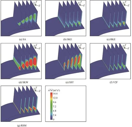
Fig.11 Contour of normal Reynolds stress incidence.

3.2.Turbulence characteristic analysis

The RANS approach requires that the Reynolds stresses are appropriately modeled in turbulence models.Except for RSM model,the other six turbulence models used in this study employ the Boussinesq hypothesis to relate the Reynolds stresses to the mean velocity gradients(referring to Eq.(3)),also called linear eddy viscosity turbulence models.If a turbulence model can predict Reynolds stress accurately,it will provide reasonable mean results on turbulence flow field.Moreover,turbulence characteristics,like turbulence viscosity and turbulent anisotropy,are considered differently in these turbulence models.Analyzing the results of turbulent characteristics is helpful to get more information about the performance of these turbulence models and can contribute to the modification of the turbulence models.

Fig.11 indicates that the Reynolds stress must be high at the corner region because the velocity fluctuation is obvious in this region.The streamwise normal stressshows the high-valued region at the corner in the seven turbulence models.This indicates that the streamwise velocity fluctuation is highly distinct at the corner separating region.However,the high-valued areas ofin these turbulence models are quite different.Thehigh-valued areas in RSM,SKE,RKE and V2F models are small and locate near the blade suction surface.By contrast,the high-valued area in SKW,SST and SA models are large and gradually move away from the blade suction surface.This phenomenon shows that these three models over predict the corner separation region and estimate stronger streamwise velocity fluctuation.The distributions of span wise and pitchwise normal stressand(not shown here)are similarto those ofItcan befound thatCompared with the shear stress shown in Fig.12,normal stress gives mainly contribution to the turbulence fluctuation because the scale of normal stress is significantly higher than that of shear stress.

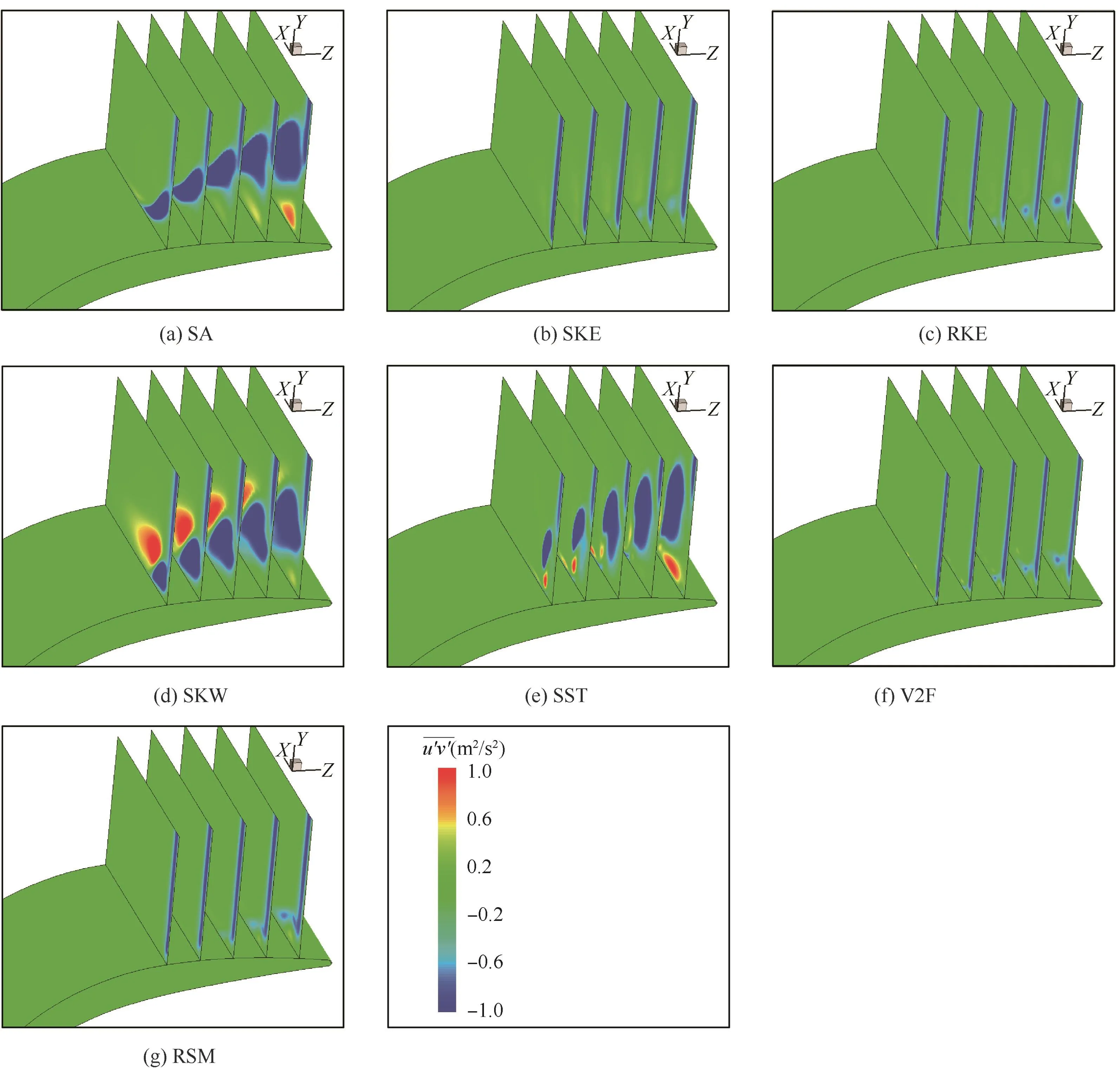
Fig.12 Contour of shear Reynolds stress u′v′at 0°incidence.

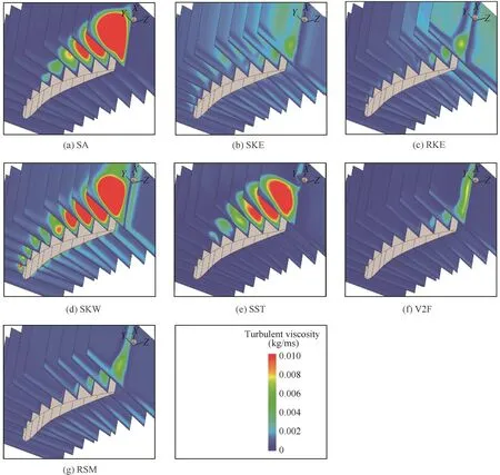
Fig.13 Contour of turbulence viscosity at 0°incidence.

Fig.12 demonstrates that the Reynolds shear stressu′v′reveals different distributions in the seven turbulence models.The high-valued areas of shear stress in V2F,SKE,RKE and RSM models are small and close to the endwall.This observation provides a vivid contrast to the results of SA,SKW and SST models.Two high-valued shear stress regions are observed in SKW model.This indicates that the shear stress is very active at the corner separating region.One shear stress core near the endwall is negative,whereas the other is positive.The high-valued shear stress regions in SST model and SA model are very distinct and the location of shear stress core is located away from suction surface of the blade.The distribution of the other two Reynolds shear stressand(not shown here)are similar to that ofand it is found

The preceding analysis verifies that SA,SKW and SST models overestimate the corner separation in the PVD cascade.The turbulent viscosity of these models is significantly larger than the results of V2F,SKE,RKE and RSM models shown in Fig.13.This finding is consistent with the analysis of Reynolds stress.When the Reynolds stress at corner region is higher,the velocity fluctuation is stronger,which in turn leads to high turbulence viscosity.

Another important turbulent characteristic is turbulent anisotropy,which is hardly to be considered correctly in the linear eddy viscosity turbulence models.It may be one reason why the linear eddy viscosity turbulence models could not predict corner separation correctly.As the turbulence models predict different Reynolds stress distributions in corner separation region,the predicted turbulent anisotropy should be different.The analysis of turbulent anisotropy in the corner region can provide information on assessing the performance of these turbulence models.

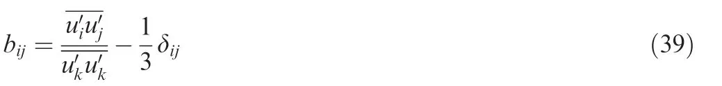
The Lumley triangle47is proven to be a useful tool to study turbulent anisotropy.Lumley found the turbulent anisotropy can be derived from Reynolds stress tensorby subtracting the isotropic partwhich is

The non-dimensional form of the anisotropy tensor bijis given by

The tensor bijhas three scalar invariants.For incompressible flows the first invariant equals 0,the second invariant(η)and third invariant(ξ)are expressed as

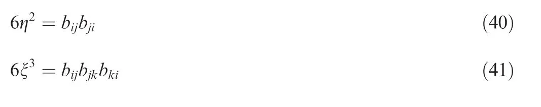
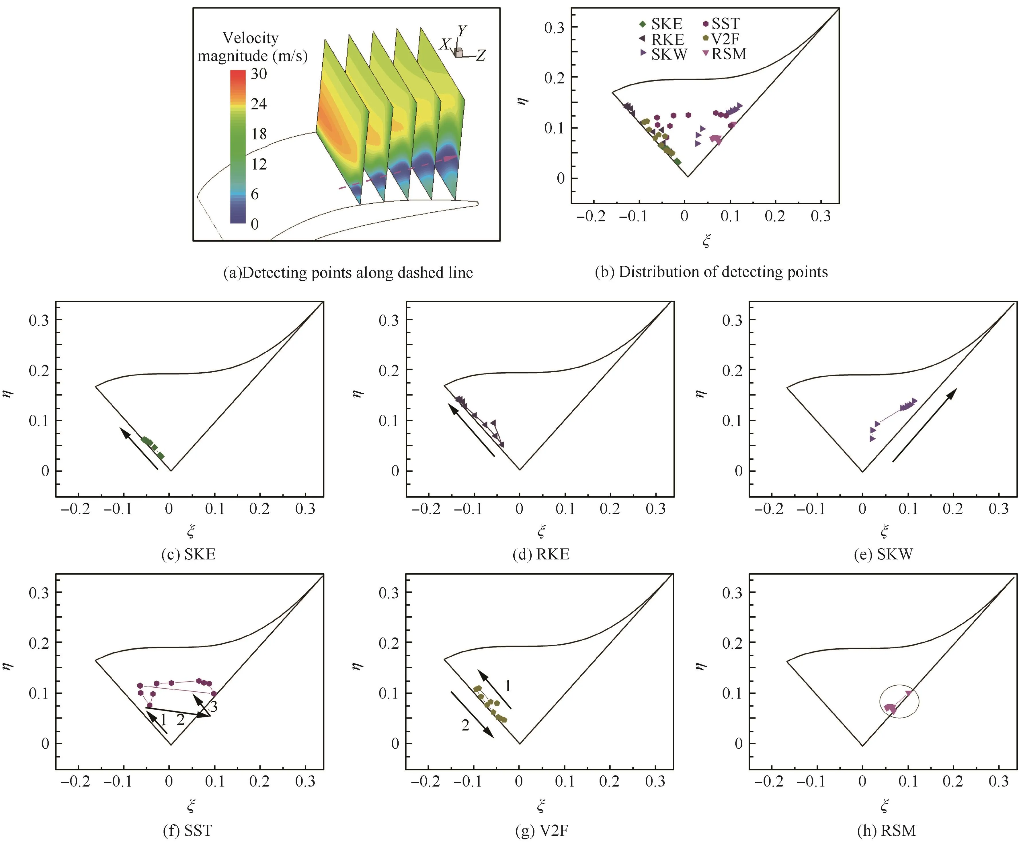
Fig.14 Anisotropy invariant map at 0°incidence.

The state of turbulence in a flow can be displayed with respect to its anisotropy by cross-plotting η and ξ.The η and ξ invariants should settle in a triangle map for real physical turbulence flow.The left line of triangle describes axisymmetric turbulence in which one direction of velocity fluctuations is weaker than the other two.This is referred to as''disklikequot;type of turbulence.In contrast,the right line of triangle is characterized by one fluctuating component which dominates over the other two.It is called''rodlikequot;turbulence.The curve edge of the triangle represents 2D turbulence.Turbulence tends to be isotropic when the point is close to the original point.

In this study,the invariants η and ξ are calculated from the line extracted in the corner region as shown in Fig.14(a).The distribution of the points is shown below.The points in the RSM model gather near the right lines of the triangle which indicate that the turbulence type is''rodlikequot;.The point distribution in SKE and SKW models varies from each other.The points in SKE model are located along the left line of the triangle,whereas those in the SKW develop along the right line.The turbulence type is''disklikequot;in the SKE model and it is''rodlikequot;in SKW model.The result of RKE model is similar to the results of SKE model.Points in V2F model move away from the origin point along the left line and then return close to the origin point.This indicates the turbulence tends to be anisotropic firstly and turns to be isotropic at the end.The results of RSM,SKE,RKE,SKW and V2F models are along the right or the left line of the triangle and turbulence types are axisymmetric.By contrast,the points in the SST model scatter within the triangle,thus the turbulence is considered anisotropic in the results of the SST model.

4.Conclusions

In this study,numerical study of corner separation in a linear highly loaded PVD compressor cascade has been investigated using seven frequently used turbulence models in FLUENT.The computational results of seven turbulence models,including Spalart–Allmaras model,standard k–ε model,realizable k–ε model,standard k–ω model,shear stress transport k–ω model,v2–f model and the Reynolds stress model,are carefully discussed and analyzed with published experimental data.The conclusions are drawn as follows:

(1)In the steady simulations,all the RANS approaches predict various scales and topologies for 3D corner separation region.At-7°incidence,the corner separation flow is weak in the cascade and these seven turbulence models except standard k–ω model can provide satisfactory results on mean flow.At 0°incidence,3D corner separation gets strong,the discrepancies in these RANS models become obvious.Among these models,the standard k–ε model,realizable k–ε model,v2–f model and the Reynolds stress model can still predict reasonable results on the mean flow,and the Reynolds stress model shows best performance;whereas the Spalart–Allmaras model,standard k–ω model and shear stress transport k–ω model overestimate the corner separation.

(2)The distribution of Reynolds stress is quite different among the results of various turbulence models.Normal Reynolds stress significantly contributes to velocity fluctuation.Three components of the shear stresses are not in the same magnitude.The Spalart–Allmaras model,standard k–ω model and shear stress transport k–ω model overestimate the Reynolds stress at the corner region.By contrast,the other turbulence models can provide relatively reasonable results.

(3)Turbulence anisotropy is explored in the study.In the corner region,the turbulence becomes more anisotropic with the development of corner separation.The standard k–ε model,realizable k–ε model,standard k–ω model,v2–f model and Reynolds stress model are along the left line or the right line of the Lumley triangle and this indicates that turbulence type is axisymmetric''dislikequot;or''rodlikequot;,whereas the points in shear stress transport k–ω model are scattered in the triangle.The turbulence anisotropy for modifying turbulence models needs further study in corner separation.

Acknowledgements

This work was supported by the National Natural Science Foundation of China(No.51376001,No.51420105008,No.51306013,No.51136003),the National Basic Research Program of China(2012CB720205,2014CB046405),the Beijing Higher Education Young Elite Teacher Project,and the Fundamental Research Funds for the Central Universities.The work is also supported by the Innovation Foundation of BUAA for Ph.D.Graduates.The authors would like to thank Whittle Laboratory and Rolls-Royce Plc for providing their experimental results.

1.Lei VM,Spakovszky ZS,Greitzer EM.A criterion for axial compressor hub-corner stall.J Turbomach 2008;130(3):031006–10.

2.Denton JD.Loss mechanisms in turbomachines.J Turbomach 1993;115:621–56.

3.Schulz HD,Gallus HE.Experimental investigation of the three dimensional flow in an annular compressor cascade.J Turbomach 1988;110(4):467–78.

4.Guo S,Lu HW,Chen F,Wu CJ.Vortex control and aerodynamic performance improvement of a highly loaded compressor cascade via inlet boundary layer suction.Exp Fluids 2013;54:1570.

5.Zhang HD,Wu Y,Li YH,Lu HW.Experimental investigation on a high subsonic compressor cascade flow.Chin J Aeronaut 2015;28(4):1034–43.

6.Scillitoe AD,Tucker PG,Adami P.Evaluation of RANS and ZDES methods for the prediction of three-dimensional separation in axial flow compressors.Montre´al:ASME;2015.Report No.:GT2015-43975.

7.Liu YW,Yan H,Lu LP.Numerical study of the effect of secondary vortex on three-dimensional corner separation in a compressor cascade.Int J Turbo Jet Eng 2015.Available from:http://dx.doi.org/10.1515/tjj-2014-0039.

8.Guo S,Chen SW,Lu HW,Song YP,Chen F.Enhancing aerodynamic performances of a high-turning compressor cascade via boundary layersuction.SciChina Tech Sci2010;53(10):2748–55.

9.Gmelin C,Thiele F,Liesner K,Meyer R.Investigations of secondary flow suction in a high speed compressor cascade.Vancouver:ASME;2011.Report No.:GT2011-46479.

10.Choi M.Effects of circumferential casing grooves on the performance of a transonic axial compressor.Int J Turbo Jet Eng 2015;32(4):361–71.

11.Liu YW,Sun JJ,Lu LP.Corner separation control by boundary layer suction applied to a highly loaded axial compressor cascade.Energies 2014;7(12):7994–8007.

12.Lakshminarayan B.Fluid dynamics and heat transfer of turbomachinery.New York:A Wiley-Interscience Publication;1996.p.322–7.

13.Spalart PR.Detached-eddy simulation.Annu Rev Fluid Mech 2009;41:181–202.

14.Menter F,Egorov Y.The scale-adaptive simulation method for unsteady turbulent flow predictions.Part 1:theory and model description.Flow Turbul Combust 2010;85(1):113–38.

15.Castagna J,Yao YF,Yao J.Direct numerical simulation of a turbulentflow over an axisymmetric hill.Comput Fluids 2014;95:116–26.

16.Zhang HD,Yan C,Ye TH,Zhang JM,Chen YL.Large eddy simulation of unconfined turbulent swirling flow.Sci China Tech Sci 2015;58(10):1731–44.

17.Liu J,Sun HS,Liu ZT,Xiao ZX.Numerical investigation of unsteady vortex breakdown past 80°/65°double-delta wing.Chin J Aeronaut 2014;27(3):521–30.

18.Wang YF,Chen F,Liu HP,Chen HL.Large eddy simulation of unsteady transitional flow on the low-pressure turbuine blade.Sci China Tech Sci 2014;57(9):1761–8.

19.Spalart PR.Philosophies and fallacies in turbulence modeling.Prog Aerosp Sci 2015;74:1–15.

20.Spalart PR.Strategies for turbulence modelling and simulations.Int J Heat Fluid Flow 2000;21:252–63.

21.Dunham J.CFD validation for propulsion system components.Neuilly-sur-Seine:AGARD;1998.Report No.:AR-355.

22.Liu YW,Yu XJ,Liu BJ.Turbulence models assessment for largescale tip vortices in an axial compressor rotor.J Propul Power 2008;24(1):15–25.

23.Vijiapurapu S,Cui J.Performance of turbulence models for flows through rough pipes.Appl Math Model 2010;34:1458–66.

24.Balabel A,Hegab AM,Nasr M,Samy El-Behery M.Assessment of turbulence modeling for gas flow in two-dimensional convergent–divergent rocket nozzle.Appl Math Model 2011;35:3408–22.

25.Liu YW,Lu LP,Fang L,Gao F.Modification of Spalart–Allmaras model with consideration of turbulence energy backscatter using velocity helicity.Phys Lett A 2011;375(24):2377–81.

26.Heschl C,Inthavong K,Sanz W,Tu J.Evaluation and improvements of RANS turbulence models for linear diffuser flows.Comput Fluids 2013;71:272–82.

27.Ma L,Lu LP,Fang J,Wang QH.A study on turbulence transportation and modification of Spalart–Allmaras model for shock-wave/turbulent boundary layer interaction flow.Chin J Aeronaut 2014;27(2):200–9.

28.Liu YW,Yan H,Lu LP.Investigation of corner separation in a linear compressor cascade using DDES.Montréal:ASME;2015.Report No.:GT2015-42902.

29.Gbadebo SA,Cumpsty NA,Hynes TP.Three-dimensional separations in axial compressors.J Turbomach 2005;127(2):331–9.

30.Fluent 6.3 User's Guide.Fluent Documentation,Fluent Inc,2006.

31.Spalart PR,Allmaras SR.A one-equation turbulence model for aerodynamic flows.Reno:AIAA;1992.Report No.:AIAA-92-0439.

32.Spalart PR,Shur M.On the sensitization of turbulence models to rotation and curvature.Aerosp Sci Technol 1997;5:297–302.

33.Launder BE,Spalding DP.The numerical computation of turbulent flows.Comput Method Appl Mech 1974;3:269–89.

34.Launder BE,Sharma BI.Application of the energy-dissipation model of turbulence to the calculation of flow near a spinning disc.Lett Heat Mass Transfer 1974;1:131–8.

35.Shih TH,Liou WW,Shabbir A.A new k–ε eddy-viscosity model for high Reynolds number turbulent flows-model development and validation.Comput Fluids 1995;24(3):227–38.

36.Wilcox DC.Turbulence modeling for CFD.San Diego:DCW Industries;2006.p.124–36.

37.Menter FR.Two-equation eddy-visocity turbulence models for engineering applications.AIAA J 1994;32(8):1598–605.

38.Durbin PA.Near-wall turbulence closure modeling without damping functions.Theor Comput Fluid Dyn 1991;3:1–13.

39.Durbin PA.Separated flow computations with the k–ε–v2model.AIAA J 1995;33(4):659–64.

40.Behnia M,Parneix S,Shabany Y.Numerical study of turbulent.Int J Heat Fluid Flow 1999;20:1–9.

41.Launder BE,Reece GJ,Rodi W.Progress in the development of a Reynolds-stress turbulence closure.J Fluid Mech 1975;3(68):537–66.

42.Gibson MM,Launder BE.Ground effects on pressure fluctuations in the atmospheric boundary layer.J Fluid Mech 1978;86:491–511.

43.Smirnov PE,Menter FR.Sensitization of the SST turbulence model to rotation and curvature by applying the Spalart–Shur correction term.J Turbomach 2009;131:0410104.

44.Gbadebo SA,Cumpsty NA,Hynes TP.Interaction of tip clearance flow and three-dimensional separations in axial compressors.J Turbomach 2007;129(4):679–85.

45.Gbadebo SA,Cumpsty NA,Hynes TP.Control of three-dimensional separations in axial compressors by tailored boundary layer suction.J Turbomach 2008;130(1):011004–8.

46.Gbadebo SA,Hynes TP,Cumpsty NA.Influence of surface roughness on three-dimensional separation in axial compressors.J Turbomach 2004;126(4):455–63.

47.Lumely J.Computational modeling of turbulent flows.Adv Appl Math 1978;18:123–76.

Liu Yangweiis currently an associate professor in the School of Energy and Power Engineering,Beihang University.His major research interests include CFD,complex flow mechanism and flow control in turbomachinery.

Yan Haois a Ph.D.candidate in Beihang University,China.His research focuses on the complex flow in compressor cascade.

Liu Yingjieis currently a senior engineer in AVIC Academy of Aeronautic propulsion technology.Her major research interests include CFD,LES and numerical simulation of combustion.

Lu Lipengis currently a professor in the School of Energy and Power Engineering,Beihang University.His major research interests include turbulence,CFD and turbomachinery.

Li Qiushiis currently a professor in the School of Energy and Power Engineering,Beihang University.His major research interests include turbomachinery,vortex aerodynamic and flow instability.

14 May 2015;revised 30 June 2015;accepted 6 January 2016

Available online 10 May 2016

Compressor cascade;

Corner separation;

Turbomachinery CFD;Turbulence anisotropy;

Turbulence models

Ⓒ2016 Production and hosting by Elsevier Ltd.on behalf of Chinese Society of Aeronautics and Astronautics.This is an open access article under the CC BY-NC-ND license(http://creativecommons.org/licenses/by-nc-nd/4.0/).

*Corresponding author at:Collaborative Innovation Center of Advanced Aero-Engine,Beihang University,Beijing 100083,China.Tel.:+86 10 82316455.

E-mail addresses:liuyangwei@126.com(Y.Liu),yanhaovsdami@163.com(H.Yan),liuyingjie@buaa.edu.cn(Y.Liu),lulp@buaa.edu.cn(L.Lu),liqs@buaa.edu.cn(Q.Li).

Peer review under responsibility of Editorial Committee of CJA.