Delving into the relationship between autumn Arctic sea ice and central-eastern Eurasian winter climate

WANG Shao-Yinand LIU Jiping

aState Key Laboratory of Numerical Modeling for Atmospheric Sciences and Geophysical Fluid Dynamics， Institute of Atmospheric Physics， Chinese Academy of Sciences， Beijing， China；bCollege of Earth Science， University of the Chinese Academy of Sciences， Beijing， China；cDepartment of Atmospheric and Environmental Sciences， University at Albany， State University of New York， Albany， NY， USA

Delving into the relationship between autumn Arctic sea ice and central-eastern Eurasian winter climate

WANG Shao-Yina，band LIU Jipingc

aState Key Laboratory of Numerical Modeling for Atmospheric Sciences and Geophysical Fluid Dynamics， Institute of Atmospheric Physics， Chinese Academy of Sciences， Beijing， China；bCollege of Earth Science， University of the Chinese Academy of Sciences， Beijing， China；cDepartment of Atmospheric and Environmental Sciences， University at Albany， State University of New York， Albany， NY， USA

Whether recent Arctic sea ice loss is responsible for recent severe winters over mid-latitude continents has emerged as a major debate among climate scientists owing to short records of observations and large internal variability in mid- and high-latitudes. In this study， the authors divide the evolution of autumn Arctic sea ice extent during 1979-2014 into three epochs， 1979-1986 （high）， 1987-2006（moderate）， and 2007-2014 （low）， using a regime shift identifcation method. The authors then compare the associations between autumn Arctic sea ice and winter climate anomalies over central and eastern Eurasia for the three epochs with a focus on extreme events. The results show robust and detectable signals of Arctic sea ice loss in weather and climate over western Siberia and East Asia. Associated with sea ice loss， the latitude （speed） of the jet stream shifts southward （reduces），the wave extent amplifes， and blocking high events increase over the Ural Mountains， leading to increased frequency of cold air outbreaks extending from central Asia to northeast China. These associations bear a high degree of similarity to the observed atmospheric anomalies during the low sea ice epoch. By contrast， the patterns of atmospheric anomalies for the high sea ice epoch are diferent from those congruent with sea ice variability， which is related to the persistent negative phase of the Arctic Oscillation.

ARTICLE HISTORY

Revised 15 April 2016

Accepted 29 April 2016

Arctic sea ice； regime shift；climate； extreme events

北极海冰的快速减少是否已经显著地影响了最近中纬度大陆冬季极端天气气候事件引起了气候学家的广泛争论。问题的争论是来源于观测数据的年限很短以及中高纬度复杂的内部变率。在本研究中，采用气候突变检测的方法，我们将秋季海冰覆盖面积的变化分为三个阶段：1979-1986（高海冰阶段），1987-2006（海冰缓慢减少阶段）和2007-2014（海冰快速减少阶段）。然后，我们分析了与每一个阶段秋季海冰变化相联系的中-东欧亚地区冬季气候（尤其极端天气事件）是什么。结果表明北极海冰减少对西伯利亚西部和东亚极端天气事件影响的信号是稳健可测的。伴随着海冰的快速减少，高低空急流速度的减弱和急流位置的南移；波动振幅的加强、乌拉尔山阻塞频率的增多。这些导致了寒潮事件从亚洲中部到中国东北部地区显著增多。并且，与北极海冰的快速减少相关的环流异常与观测到的环流异常基本一致。相反地，在高海冰阶段，与海冰相关的环流异常和观测的异常并不一致。这个阶段的环流异常是与北极涛动处于持续的负位相有关的。

1. Introduction

For the past few decades， Arctic sea ice has experienced signifcant changes in the context of amplifed warming in the Arctic （e.g. Cavalieri and Parkinson 2012）. Satellite records show that Arctic sea ice extent has been decreasing in all months， with the largest loss in September （e.g. Stroeve et al. 2012）. The decline of Arctic sea ice has accelerated since the 2000s， reaching a record low in 2012，recovering slightly in 2013 and 2014， and reaching the fourth lowest minimum in 2015. The decreasing Arctic sea ice since the late 1970s is a consequence of the combination of anthropogenic forcing and natural variability （e.g. Overland and Wang 2010； Swart 2015）. Arctic sea ice loss reduces surface albedo and allows more solar radiation to be absorbed by the ocean and released into the atmosphere in winter， amplifying Arctic warming and potentially having remote efects on mid-latitude weather and climate（e.g. Vihma 2014）.

Recent research concerns the possible links between Arctic sea ice changes and midlatitude weather and climate. Some studies （Francis and Vavrus 2012； Liu et al. 2012） have linked Arctic sea ice loss （via a weakened meridional temperature gradient and westerly winds） to a meandering jet stream that leads to prolonged and more frequent extreme events （e.g. cold surges）. Many studies have expanded on and modifed this hypothesis. For instance， based on observational data， Arctic sea ice loss has been linked to increased snow cover over northern Eurasia （e.g. Cohen et al. 2014） and cold winter extremes in the mid-latitudes （e.g. Tang et al. 2013）. Some studies（e.g. Coumou et al. 2014； Screen and Simmonds 2014） have reported amplifed mid-latitude atmospheric planetary waves in response to Arctic warming. Based on atmospheric model simulations with prescribed sea ice loss， the atmospheric response shows a weakening of the westerly winds （e.g. Kim et al. 2014； Peings and Magnusdottir 2014），which leads to severe winters in East Asia or North America（Mori et al. 2014； Kug et al. 2015）.

Meanwhile， a number of studies have questioned this hypothesis. The arguments include natural variability driving extreme weather events， and no signifcant change in the jet stream. Based on reanalysis data， a few studies have shown there to be no signifcant long-term trend in the jet stream and blocking events over North America， owing to diferent defnitions of the metrics involved and short records of observations （Barnes 2013； Woollings， Harvey，and Masato 2014）. In model simulations， the atmospheric response is sometimes weak compared to atmospheric internal variability， depending on the atmospheric model used and the ensemble members （Screen et al. 2014）. Thus，the challenge remains to attribute the recent mid-latitude weather changes to either Arctic sea ice loss or natural variability （e.g. Cohen et al. 2014； Fischer and Knutti 2014）.

For Eurasia， a number of studies have shown that the reduction of autumn Arctic sea ice， especially that of the Barents-Kara Seas， is closely linked to the following winter climate， either through a negative Arctic Oscillation like response or an intensifed Siberian high （e.g. Mori et al. 2014； Gao et al. 2015）. However， a comprehensive analysis of the jet stream， wave amplitude， and extreme events over central and eastern Eurasia is lacking in these studies. In this study， therefore， we provide a more detailed picture of the link between Arctic sea ice change and the weather and climate over central and eastern Eurasia， with a focus on extreme events.

2. Data and methods

The datasets used in this study include: （1） the Arctic sea ice extent index， which is defned as the total area of the Arctic covered by at least 15% sea ice concentration， obtained from the National Snow and Ice Data Center，which is retrieved from the SMMR/SSMI satellites based on the NASA team algorithm （Comiso and Nishio 2008）；（2） the monthly and daily SLP， surface air temperature， zonal winds， and 500-hPa geopotential height from ERA-Interim，with a horizontal resolution of 1.5° （Dee et al. 2011）； and （3）Arctic Oscillation （AO） indices obtained from http://www. esrl.noaa.gov/psd/data/climateindices/list/. The common period for the above datasets is from 1979 to 2014， and seasonal anomalies are obtained by removing the climatology. We calculate the autumn average （September-October-November） for the sea ice extent index and the winter average （December-January-February） for the other datasets.

A climatic regime shift is often considered as a rapid reorganization of climate from one relatively stable state to another. Several methods have been proposed to detect regime shifts for atmospheric and oceanic variables （e.g. Rodionov 2004）. Here， we use a scheme developed by Rodionov （2004） to identify possible regime shifts in the time series of the autumn Arctic sea ice extent. This scheme is based on a sequential data processing technique to determine the timing of the regime shifts. The identifcation of a regime shift is based on computing the regime shift index， which is an indicator of the hypothetical mean level for the new regime. The shift points are identifed if the diference of the mean level between the new state and the previous state is statistically signifcant， based on the Student’s t-test （Overland et al. 2008）. The advantage of this scheme is that it does not require a prior hypothesis on the timing of regime shifts （Rodionov 2006）. Here， the signifcant level and cut-of length （analogy in cut-of frequency in fltering） used in the method is set to 0.05 and 10 years.

The composite of winter atmospheric anomalies for each sea ice regime is calculated at each grid point by （1）regressing winter atmospheric anomalies on the autumn sea ice extent index for 1979-2014， （2） multiplying the resulting regression coefcients by the autumn sea ice extent index， and （3） averaging the values from （2） for diferent sea ice regimes （detected by the regime shift method）. The statistical signifcance of the regression is calculated using the Student’s t-test. Note that caution is needed when carrying out regression between two variables having trends. Thus， we also repeat the above composite analysis using the detrended data. Comparisons between the two analyses help us to determine the relative role of interannual and long-term variability of autumn sea ice in the observed atmospheric anomalies.

3. Results

3.1. Arctic sea ice regime shifts

Figure 1.Standardized autumn （average of September， October， and November） sea ice extent （ASIE） index （red line）， standardized and detrended ASIE index （green line）， standardized winter AO index （blue line）， and sea ice regimes （black line）.

Figure 1 shows the standardized autumn Arctic sea ice extent （ASIE， red line） from 1979 to 2014. Superimposed on strong interannual variability， the ASIE shows a significant downward trend at a rate of ～6.7% per year （＞99% confdence level）. However， the decrease of Arctic sea ice is not linear， characterized by periods of oscillation. We apply the aforementioned sequential t-test method to the ASIE to detect the possible regime shifts. The results suggest that regime shifts occurred in 1987 and 2007. Hence， we defne three sea ice regimes （horizontal black lines in Figure 1）: （1） 1979-1986 （high sea ice epoch， hereafter referred to as HSI）； （2） 1987-2006 （moderate sea ice epoch， hereafter referred to MSI） and 2007-2014 （low sea ice epoch， hereafter referred to as LSI）. During the HSI， the ASIE shows some fuctuation with a mean of 9.40 million km2， but no trend. Compared to the HSI， the ASIE exhibits a gradual decrease at a rate of about 0.07 million km2yr-1during the MSI， with a mean of 8.7 million km2. A sharp decline of sea ice occurred in 2007， reaching a record low in 2012， and there has been no signifcant recovery of sea ice since 2007. This leads to a mean of 7.5 million km2during the LSI， which is 20.2% less than that of the HSI. The identifed regime shifts here are generally consistent with recent studies. Curry （see http://judithcurry. com/2011/03/19/pondering-the-arctic-ocean-part-i-climate-dynamics/ for details） pointed out that it is instructive to interpret the record in the context of a （qualitative）change point analysis， defned by changes in trend， mean value， amplitude of the annual cycle， and interannual variability. The Arctic sea ice extent during 1979-1988 is characterized by little trend， and consistent interannual variability in the amplitude of the seasonal cycle. Livina and Lenton （2013）， through detecting multi-modality of the seasonal cycle of sea ice area， suggested that the year 2007 was a tipping point. Meanwhile， Overland et al.（2012） showed that the summer atmospheric circulation pattern in the Arctic for 2007-2012 was diferent from that of the previous decade.

Figure 2 （upper panel） shows the composite of the observed winter SLP anomalies for the aforementioned three epochs. The observed SLP anomalies during the HSI exhibit an above-normal pressure in the high-latitudes and a below-normal pressure in the mid-latitudes （Figure 2（a1））. However， signifcant SLP anomalies are only located in the mid-latitudes of the western North Pacifc， which indicates an intensifcation and southwestward expansion of the Aleutian low. In contrast， the pressure pattern during the MSI shows large （small） negative （positive） SLP anomalies north （south） of ～50°N， but the SLP anomalies are not statistically signifcant （Figure 2（a2））. During the LSI， the SLP pattern in general is opposite to that of the MSI. The SLP is substantially higher over Siberia， as well as the ocean to the east of Japan， which is accompanied by lower SLP over central and southern Asia （Figure 2（a3））.

During the HSI， the composite of the SLP anomalies regressed on the ASIE shows positive （negative） pressure anomalies north （south） of ～40°N， with signifcant anomalies east of 110°E （Figure 2（b1））， which is diferent from the observed SLP anomalies during the HSI （Figure 2（a1））. This is also true for the detrended data. Hence，the observed SLP anomalies during the HSI cannot be attributed to sea ice variability. Associated with gradually decreased sea ice， large parts of Siberia are dominated by signifcant negative SLP anomalies （Figure 2（b2））， which are similar to those of Figure 2（a2）， but the magnitude is smaller. Note that the small magnitude is largely due to the ASIE evolving from positive to negative phase during the MSI， resulting in the cancellation of the regression before and after the phase transition. This suggests that sea ice variability during the MSI plays a certain role in the observed SLP anomalies. In contrast， the SLP pattern associated with low sea ice during 2007-2014（Figure 2（b3）） resembles that of Figure 2（a3）， indicating that the rapid decline of sea ice is closely related tothe observed strengthening of the Siberian high. The composite of the detrended SLP anomalies regressed onto the detrended ASIE during the LSI （Figure 2（c3））is similar to that of Figure 2（a3） and （b3）， even though signifcant areas are confned to central Siberia （positive）and southwestern Asia （negative）. This suggests that the observed pressure anomalies in these areas are closely associated with interannual sea ice variability， while the other signifcant relationships in Figure 2（b2） may arise through combined decreasing sea ice trend and hemispheric warming. Thus， associated with the reduced autumn Arctic sea ice， the Siberian high is intensifed. This is consistent with the results from recent numerical experiments using atmospheric models forced with prescribed sea ice changes （Honda， Inoue， and Yamane 2009；Mori et al. 2014）. They showed that anomalously low sea ice cover in the Barents-Kara Seas in summer to autumn（Honda， Inoue， and Yamane 2009） and September （Mori et al. 2014） leads to a strengthening of the Siberian high.

Figure 2.Composite SLP anomalies （units: hPa） for three sea ice epochs: （a1-a3） observed SLP anomalies in （a1） 1979-1986， （a2）1987-2006， and （a3） 2007-2014； （b1-b3） as in （a1-a3） but for composite anomalies regressed on the ASIE； （c1-c3） as in （a1-a3） but for composite anomalies regressed on the detrended ASIE.

3.2. Extreme event metrics

Extreme weather events have signifcant consequences on society and ecosystems， and thus their changes are presumably more important than the mean state. Here，we calculate the metrics of the jet stream， Rossby wave，blocking events， and cold air outbreaks over central and eastern Eurasia. The extreme events used are defned using daily ERA-Interim data.

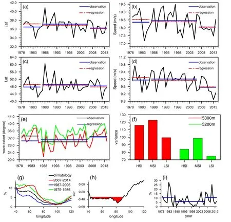
Figure 3.Two measures of the observed East Asian region jet latitude and speed. （a， b） upper-level jet latitude and jet speed （Archer and Caldeira 2008）； （c， d） lower-level jet latitude and jet speed （Woollings， Hannachi， and Hoskins 2010）. Blue lines denote the averaged jet latitude or speed over three sea ice epochs， and red dashed lines are the same as the blue lines but for jet latitude or speed regressed on the sea ice extent. Panel （e） shows the wave extent time series for two isopleth （5300 m， red， and 5200 m， green）， and （f） the wave extent variance， for the three sea ice epochs. The black lines in （e） denote the averaged wave extent over the three sea ice epochs （here， the wave extent of 5300 m is presented）. （g） 1D blocking index for the climatology and three sea ice epochs. （h） Corresponding correlation coefcients with the ASIE （red area indicates the confdence level exceeds 95%）. （i） Time series of the Urals blocking index， which is defned as the zonal-averaged blocking of the Ural Mountains region （40-70°E）.

Figure 3 （upper panel） shows the upper level jet latitude and speed. The upper level jet is defned as the mass weighted zonal wind averaged from 400 to 100 hPa， following Archer and Caldeira （2008）； and the jet latitude is calculated using Archer and Caldeira （2008， Equation（3）） for the latitude band between 15°N and 80°N. At the upper level， the averaged jet latitude moves equatorward by ～0.87° during the LSI compared to that of the MSI， but the jet latitude during the HSI falls between that of the LSI and MSI （Figure 3（a）， blue line）. The jet speed time series show large variabilities and， for the LSI， the jet speed with a mean of about 18.1 m s-1is slower than that of the MSI and HSI （Figure 3（b）， blue line）. The composite of the upper jet regressed on the ASIE （Figure 3（a） and （b）， red line）closely matches the observed values （blue line） for the MSI and LSI. However， for the HSI， the observed jet latitude and speed are inconsistent with the regression. This suggests that other processes might play more important roles in modulating the upper jet during the HSI. Figure 3（the second panel） shows the lower level jet latitude and speed. The lower jet speed over East Asia is defned as the maximum westerly wind speed of vertically averaged（925-700 hPa） zonal wind， following Woollings， Hannachi，and Hoskins （2010）； and the jet latitude is defned as thelatitude at which the maximum is found. The eddy-driven jet latitude and speed have moderate correlation with the upper jet latitude and speed （r = 0.63 for latitude and r = 0.24 for speed）. There is no distinct diference in the jet latitude for the three epochs， but the jet latitude has a signifcant downward trend during 1987-2014 （-0.08° yr-1；＞95% confdence level）. Like the upper jet speed， the lower jet speed for the LSI is weaker than that of the MSI and HSI （Figure 3（d）， blue line）. The composite of the lower jet regressed on ASIE （Figure 3（d）， red line） is consistent with the observed value for the LSI （Figure 3（d）， blue line）， which is similar to that of the upper jet. The more equatorward and weaker jet associated with the reduction in sea ice means enhanced and broader meridional meanders in the mid-latitudes， producing a wave-like pattern of troughs and ridges （e.g. Liu et al. 2012）. The eddy-driven jet interacts with the mid-latitude Rossby waves and blocking.

Figure 3 （the third panel） shows the wave extent and its variance for the three epochs. The wave extent is defned as the diference between the daily maximum and minimum latitude of the isopleth of 5200 and 5300 m. The wave extent of 5200 and 5300 m for the LSI （36.3° and 33.2°） is substantially larger than that of the MSI （34.1° and 29.9°），but the wave extent of the HSI （36.2° and 32.8°） is comparable to that of the LSI （Figure 3（e）， black line）. Moreover，the variance of the wave extent for the LSI is the smallest among the three epochs （Figure 3（f））. The composite of the wave extent regressed on the ASIE （blue line） matches the observed values （black line） well for the LSI， but for the HSI the regression is inconsistent with the observation.

Figure 3 （the fourth panel） shows the 1D blocking index， which is defned as the persistent reversal of 500-hPa geopotential height along the latitude from 15°N to 80°N （Barriopedro et al. 2006）. The climatological 1D blocking index shows a high occurrence of blocking over the Urals-Siberia region （40-70°E； Figure 3（g）， black line）. The blocking frequency for the LSI and HSI is signifcantly higher than that of the climatology between 40°E and 90°E. And the blocking frequency for the LSI is relatively higher than that of the HSI over 60-80°E. The opposite is the case for the MSI （lower than the climatology； Figure 3（g）， blue line）. The correlations between the detrended sea ice and 1D blocking index at each longitude are negative between 42°E and 90°E （＞95% confdence level； Figure 3（h）， red area）， suggesting that the reduction of sea ice is related to the increased frequency of the Urals blocking. As shown in Figure 3（i）， the frequency of the Urals blocking （defned as the averaged blocking frequency between 40°E and 70°E）shows an increasing trend since 1987. Many studies （e.g. Cheung et al. 2012） have shown the increase of the Urals blocking is associated with the enhanced East Asian winter monsoon （EAWM）. Mori et al. （2014）， using both reanalysis data and numerical experiments， also showed that the reduction in sea ice leads to more frequent Eurasian blockings， which accounts for the severe winters over the Eurasia mid-latitudes.

Figure 4 （upper panel） shows the composite of 2D blocking event anomalies for the three epochs. Here， a blocking event is defned as the daily 500-hPa geopotential height anomaly that exceeds 1 standard deviation above the winter mean for at least fve consecutive days（Thompson and Wallace 2001）. For the HSI， there is an increased frequency of blockings over western and central Siberia and a decreased frequency of blockings south of 40°N （Figure 4（a1））. The blocking pattern of the MSI tends to be out-of-phase with that of the HSI （Figure 4（a2） vs. Figure 4（a1））. By contrast， for the LSI， the blocking increases in the high-latitudes （north of 50°N） and over central and eastern China， and decreases in between （Figure 4（a3））. The composite of blocking anomalies regressed on the ASIE for the LSI is in good agreement with the observed anomaly pattern （Figure 4（a3） vs. Figure 4（b3））， but this is not the case for the HSI. Without the trend， the blocking pattern remains largely unchanged， but the magnitude is reduced （Figure 4（c3））. This suggests that the increased incidence of blockings over Siberia may arise through combined Arctic sea ice variability and amplifed Arctic warming. The blocking pattern for the LSI favors more incursions of cold air masses from the Arctic into East Asia.

Figure 4 （the fourth panel） shows the composite anomaly of cold events. A cold event is defned as the days when ERA-Interim daily minimum surface air temperature is 1.5 standard deviations below the local climatological mean （Thompson and Wallace 2001）. For the HSI， there is an increased incursion of cold air outbreaks extending from western Siberia to northern and eastern China （Figure 4（d1））. The composite cold event anomalies associated with the ASIE are diferent from those of the observation for the HSI （Figure 4（e1））. By contrast， they bear close resemblance to the observation for the LSI（Figure 4（d3） vs. Figure 4（e3））. A similar anomaly pattern is also obtained after removing the linear trend， and the areas with a signifcantly increased frequency of cold air outbreaks extend southeastward to the ocean east of Japan （Figure 4（f3））. This suggests that， corresponding to the recent sea ice loss， there are more frequent cold events associated with below-normal temperature anomalies of 2-3 °C in central Eurasia and East Asia. For the HSI， however， the regression anomaly associated with sea ice （Figure 4（e1）） is diferent from that in Figure 4（d1）. The model experiments with prescribed sea ice cover in the Barents-Kara Seas also suggest that sea ice decline tends to induce more severe cold winters in Europe and the Far East by generating stationary Rossby waves and amplifying the Siberian high （Honda， Inoue， and Yamane 2009； Mori et al. 2014）.

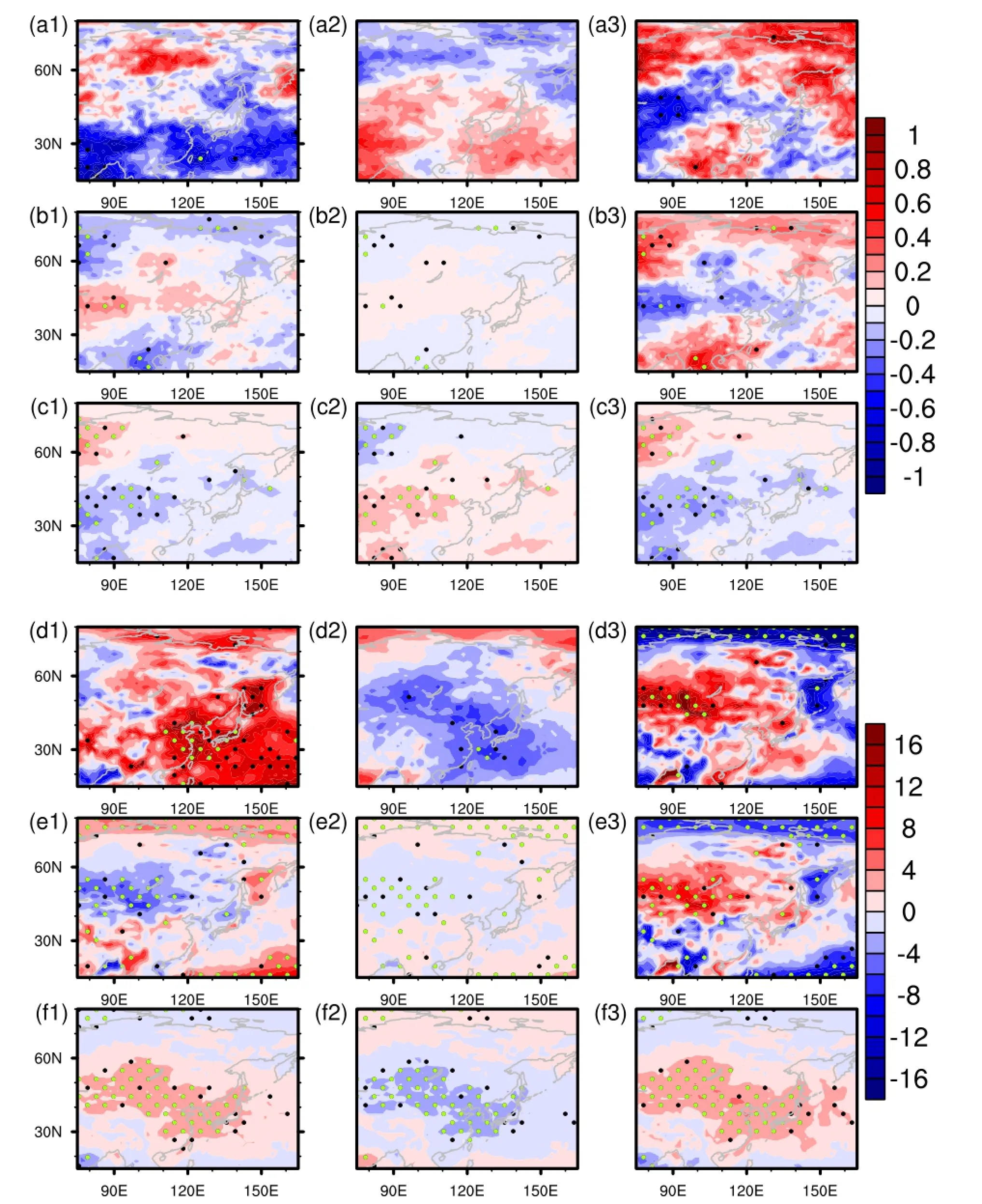
Figure 4.Composite 2D blocking anomalies for three sea ice epochs: （a1-a3） observed 2D blocking anomalies in （a1） 1979-1986， （a2）1987-2006， and （a3） 2007-2014； （b1-b3） as in （a1-a3） but for composite anomalies regressed on the ASIE； （c1-c3） as in （a1-a3） but for composite anomalies regressed on the detrended ASIE.

4. Discussion and conclusion

In this study， we take a close look at the linkages between the variability of Arctic sea ice and atmospheric circulation over central and eastern Eurasia， with a focus on extreme events.

We identify two regime shifts for the evolution of autumn Arctic sea ice extent， which occurred in 1987 and 2007. We defne three sea ice epochs and then investigate the relationship between autumn Arctic sea ice and mid-latitude extreme events for these three epochs. The Arctic sea ice loss is associated with a weaker jet stream speed and an equatorward shift of the jet stream for both the upper and lower level jets， and an amplifying wave extent. The blocking high event responses show a substantial increase over western Siberia， indicating an increase of the frequency of Urals blocking with sea ice loss. These lead to the increased frequency of cold air outbreaks in central Asia and northern China. These associations have approximately the same patterns of observed atmospheric anomalies during the low sea ice epoch. Our results show that the extreme event metrics over central and eastern Eurasia are to a large extent consistent with the Francis and Vavrus （2012） hypothesis， which indicates the recent sea ice loss has robust and detectable signals in East Asia. The model experiments prescribed by the recent sea ice loss also confrm such robust and detectable signals （Mori et al. 2014； Kug et al. 2015）.

The regressions associated with sea ice variability are generally consistent with the observed atmospheric anomalies for the MSI. However， for the HSI， the regressions associated the ASIE are diferent from the observed anomalies （e.g. Figure 2（a1） and （b1））， although they show signifcantly severe winters over southwestern Asia and the western North Pacifc （Figure 4（d1））， with a strengthened Aleutian low. The question is， what process is responsible for this inconsistency？ The AO is the dominant mode of climate variability in the Northern Hemisphere， and not only afects westerly fow， temperature， and precipitation， but also extreme events such as cold air breakouts and blocking high events （Thompson and Wallace 2001）. For the HSI， the AO remains in negative phase （Figure 1， blue line）. The persistent negative phase of the AO is concurrent with a stronger East Asian trough and an anomalous anticyclonic fow over the Urals in the mid-troposphere （Gong， Wang， and Zhu 2001； Wu and Wang 2002）， inducing the colder than normal conditions over East Asia. Thus， the increase in cold air outbreaks over the eastern Asia region may be largely related to the negative phase of the AO for the HSI. Using atmospheric reanalysis data from 1958 to 2000 （winter）， Jhun and Lee （2004） analyzed interannual and interdecadal variabilities of the EAWM associated with diferent climate modes. They found the AO is closely related to the EAWM intensity on the interdecadal time scale. The observed cold anomalies for the HSI in our study resemble the anomaly pattern for the period 1980-1986， which corresponds to the strong EAWM （Jhun and Lee 2004）. However， the recent strong EAWM epoch （2004-2012）is quite diferent to the previous （1976-1987）， which suggests the recent strong EAWM epoch is unlikely to be associated with the AO （Wang and Chen 2014）. The question is， why does the AO not play a dominant role for the LSI？ As shown in Figure 1， unlike the persistent negative phase of the AO for the HSI， it swings between negative and positive phases for the LSI.

Overall， compared to the AO， the recent sea ice loss has served as a key factor inducing the cold severe winters from central Asia to northern China. Our fndings， to some extent， corroborate the hypothesis that the decline in autumn Arctic sea ice tends to slow down and amplify the planetary waves， enhancing atmospheric blocking and more frequent southward advection of cold air masses，leading to more extreme weather events in the midlatitudes， and the signal to noise ratio of sea ice loss in East Asian atmospheric circulation is detectable and robust.

Disclosure statement

No potential confict of interest was reported by the authors.

Funding

This work was supported by the National Natural Science Foundation of China ［grant number 41176169］； the National Basic Research Program of China ［grant number 2011CB309704］.

References

Archer， C. L.， and K. Caldeira. 2008. “Historical Trends in the Jet Streams.” Geophysical Research Letters 35 （8）: L08803. doi:10.1029/2008GL033614.

Barnes， E. A. 2013. “Revisiting the Evidence Linking Arctic Amplifcation to Extreme Weather in Midlatitudes.”Geophysical Research Letters 40 （17）: 4734-4739.

Barriopedro， D.， R. Garcia-Herrera， A. R. Lupo， and E. Hernandez. 2006. “A Climatology of Northern Hemisphere Blocking.”Journal of Climate 19 （6）: 1042-1063.

Cavalieri， D. J.， and C. L. Parkinson. 2012. “Arctic Sea Ice Variability and Trends， 1979-2010.” Cryosphere 6 （4）: 881-889.

Cheung， H. N.， W. Zhou， H. Y. Mok， and M. C. Wu. 2012.“Relationship between Ural-Siberian Blocking and the East Asian Winter Monsoon in Relation to the Arctic Oscillation and the El Niño-Southern Oscillation.” Journal of Climate 25（12）: 4242-4257.

Cohen， J.， J. A. Screen， J. C. Furtado， M. Barlow， D. Whittleston，D. Coumou， J. Francis， et al. 2014. “Recent Arctic Amplifcation and Extreme mid-latitude Weather.” Nature Geoscience 7 （9）: 627-637.

Comiso， J. C.， and F. Nishio. 2008. “Trends in the Sea Ice Cover Using Enhanced and Compatible AMSR-E， SSM/I， and SMMR Data.” Journal of Geophysical Research-Oceans 113 （C2）: C02S07. doi:10.1029/2007JC004257.

Coumou， D.， V. Petoukhov， S. Rahmstorf， S. Petri， and H. J. Schellnhuber. 2014. “Quasi-resonant Circulation Regimes and Hemispheric Synchronization of Extreme Weather in Boreal Summer.” Proceedings of the National Academy of Sciences of the United States of America 111 （34）: 12331-12336.

Dee， D.， S. M. Uppala， A. J. Simmons， P. Berrisford， P. Poli，S. Kobayashi， U. Andrae， et al. 2011. “The ERA-Interim Reanalysis: Confguration and Performance of the Data Assimilation System.” Quarterly Journal of the Royal Meteorological Society 137 （656）: 553-597.

Fischer， E. M.， and R. Knutti. 2014. “Impacts: Heated Debate on Cold Weather.” Nature Climate Change 4 （7）: 537-538.

Francis， J. A.， and S. J. Vavrus. 2012. “Evidence Linking Arctic Amplifcation to Extreme Weather in Midlatitudes.” Geophysical Research Letters 39: L06801. doi:10.1029/2012GL051000.

Gao， Y. Q.， J. Sun， F. Li， S. He， S. Sandven， Q. Yan， Z. Zhang，et al. 2015. “Arctic Sea Ice and Eurasian Climate: A Review.”Advances in Atmospheric Sciences 32 （1）: 92-114.

Gong， D. Y.， S. W. Wang， and J. H. Zhu. 2001. “East Asian Winter Monsoon and Arctic Oscillation.” Geophysical Research Letters 28 （10）: 2073-2076.

Honda， M.， J. Inoue， and S. Yamane. 2009. “Infuence of Low Arctic Sea-ice Minima on Anomalously Cold Eurasian Winters.” Geophysical Research Letters 36: L08707. doi:10.1029/2008GL037079.

Jhun， J. G.， and E. J. Lee. 2004. “A New East Asian Winter Monsoon Index and Associated Characteristics of the Winter Monsoon.”Journal of Climate 17 （4）: 711-726.

Kim， B. M.， S.-W. Son， S.-K. Min， J.-H. Jeong， S.-J. Kim， X. Zhang，T. Shim， and J.-H. Yoon. 2014. “Weakening of the Stratospheric Polar Vortex by Arctic Sea-ice Loss.” Nature Communications 5: 4646. doi:10.1038/ncomms5646.

Kug， J.-S.， J.-H. Jeong， Y.-S. Jang， B.-M. Kim， C. K. Folland， S.-K. Min， and S.-W. Son. 2015. “Two Distinct Infuences of Arctic Warming on Cold Winters over North America and East Asia.”Nature Geoscience 8: 759-762.

Liu， J. P.， J. A. Curry， H. J. Wang， M. R. Song， and R. M. Horton. 2012. “Impact of Declining Arctic Sea Ice on Winter Snowfall.”Proceedings of the National Academy of Sciences of the United States of America 109 （11）: 4074-4079.

Livina， V. N.， and T. M. Lenton. 2013. “A Recent Tipping Point in the Arctic Sea-ice Cover: Abrupt and Persistent Increase in the Seasonal Cycle since 2007.” Cryosphere 7 （1）: 275-286.

Mori， M.， M. Watanabe， H. Shiogama， J. Inoue， and M. Kimoto. 2014. “Robust Arctic Sea-ice Infuence on the Frequent Eurasian Cold Winters in past Decades.” Nature Geoscience 7（12）: 869-873.

Overland， J. E.， and M. Y. Wang. 2010. “Large-scale Atmospheric Circulation Changes are Associated with the Recent Loss of Arctic Sea Ice.” Tellus Series a-Dynamic Meteorology and Oceanography 62 （1）: 1-9.

Overland， J.， S. Rodionov， S. Minobe， and N. Bond. 2008.“North Pacifc Regime Shifts: Defnitions， Issues and Recent Transitions.” Progress in Oceanography 77 （2-3）: 92-102.

Overland， J. E.， J. A. Francis， E. Hanna， and M. Y. Wang. 2012.“The Recent Shift in Early Summer Arctic Atmospheric Circulation.” Geophysical Research Letters 39: L19804. doi:10.1029/2012GL053268.

Peings， Y.， and G. Magnusdottir. 2014. “Response of the Wintertime Northern Hemisphere Atmospheric Circulation to Current and Projected Arctic Sea Ice Decline: A Numerical Study with CAM5.” Journal of Climate 27 （1）: 244-264.

Rodionov， S. N. 2004. “A Sequential Algorithm for Testing Climate Regime Shifts.” Geophysical Research Letters 31 （9）: L09204. doi:10.1029/2004GL019448.

Rodionov， S. N. 2006. “Use of Prewhitening in Climate Regime Shift Detection.” Geophysical Research Letters 33 （12）: L12707. doi:10.1029/2006GL025904.

Screen， J. A.， and I. Simmonds. 2014. “Amplifed Mid-latitude Planetary Waves Favour Particular Regional Weather Extremes.” Nature Climate Change 4 （8）: 704-709.

Screen， J. A.， C. Deser， I. Simmonds， and R. Tomas. 2014.“Atmospheric Impacts of Arctic Sea-ice Loss， 1979-2009: Separating Forced Change from Atmospheric Internal Variability.” Climate Dynamics 43 （1-2）: 333-344.

Stroeve， J. C.， M. C. Serreze， M. M. Holland， J. E. Kay， J. Malanik，and A. P. Barrett. 2012. “The Arctic’s Rapidly Shrinking Sea Ice Cover: A Research Synthesis.” Climatic Change 110 （3-4）: 1005-1027.

Swart， N. C. 2015. “Infuence of Internal Variability on Arctic Seaice Trends （Vol 5， Pg 86， 2015）.” Nature Climate Change 5 （6）: 511-511.

Tang， Q. H.， X. J. Zhang， X. H. Yang， and J. A. Francis. 2013. “Cold Winter Extremes in Northern Continents Linked to Arctic Sea Ice Loss.” Environmental Research Letters 8 （1）: 014036.

Thompson， D. W. J.， and J. M. Wallace. 2001. “Regional Climate Impacts of the Northern Hemisphere Annular Mode.” Science 293 （5527）: 85-89.

Vihma， T. 2014. “Efects of Arctic Sea Ice Decline on Weather and Climate: A Review.” Surveys in Geophysics 35 （5）: 1175-1214.

Wang， L.， and W. Chen. 2014. “The East Asian Winter Monsoon: Re-amplifcation in the mid-2000s.” Chinese Science Bulletin 59（4）: 430-436.

Woollings， T.， A. Hannachi， and B. Hoskins. 2010. “Variability of the North Atlantic Eddy-driven Jet Stream.” Quarterly Journal of the Royal Meteorological Society 136 （649）: 856-868.

Woollings， T.， B. Harvey， and G. Masato. 2014. “Arctic Warming，Atmospheric Blocking and Cold European Winters in CMIP5 Models.” Environmental Research Letters 9 （1）: 014002.

Wu， B. Y.， and J. Wang. 2002. “Possible Impacts of Winter Arctic Oscillation on Siberian High， the East Asian Winter Monsoon and Sea-ice Extent.” Advances in Atmospheric Sciences 19 （2）: 297-320.

北极海冰； 气候突变检测；气候； 极端天气事件

3 March 2016

CONTACT WANG Shao-Yin wangsy@lasg.iap.ac.cn

© 2016 The Author（s）. Published by Informa UK Limited， trading as Taylor & Francis Group.

This is an Open Access article distributed under the terms of the Creative Commons Attribution License （http://creativecommons.org/licenses/by/4.0/）， which permits unrestricted use， distribution， and reproduction in any medium， provided the original work is properly cited.