Spatiotemporal characteristics of the sea level anomaly in the Kuroshio Extension using a self-organizing map

MA Fng， DIAO Yi-Nnd LUO De-Hi

aCollege of Oceanic and Atmospheric Sciences， Ocean University of China， Qingdao， China；bKey Laboratory of Regional Climate-Environment for Temperate East Asia Key Laboratory of Regional Climate-Environment for Temperate East Asia， Chinese Academy of Sciences， Beijing， China

Spatiotemporal characteristics of the sea level anomaly in the Kuroshio Extension using a self-organizing map

MA Fanga，b， DIAO Yi-Naaand LUO De-Haib

aCollege of Oceanic and Atmospheric Sciences， Ocean University of China， Qingdao， China；bKey Laboratory of Regional Climate-Environment for Temperate East Asia Key Laboratory of Regional Climate-Environment for Temperate East Asia， Chinese Academy of Sciences， Beijing， China

Satellite altimeter SSH data in the Kuroshio Extension （KE） region gathered during the period January 1993 to December 2014 are analyzed using self-organizing map （SOM） analysis. Four spatial patterns （SOM1， SOM2， SOM3， and SOM4） are extracted， and the corresponding time series are used to characterize the variation of the sea level anomaly. Except in some individual months， SOM1 and SOM2 with single-branch jet structures appear alternately during the periods 1993—1998 and 2002—2011. However， during 1999—2001 and 2012—2014， SOM3 and SOM4 with double-branch jet structures are dominant. The sea level anomalies exhibit interannual variations， while the KE stream demonstrates decadal variation. For SOM1， the change in the KE path is less evident， although the KE jet is strong and narrow. For SOM2， the KE jet is weakened and widened and its jet axis moves towards the southwest. Compared with the SOM3， for SOM4 the trough and ridge in the upstream KE region are deeper in the northeast—southwest direction， and accompanied by a jet weakening and splitting. This study shows that SOM analysis is a useful approach for characterizing KE variability.

ARTICLE HISTORY

Revised 25 May 2016

Accepted 2 June 2016

Sea level anomaly； selforganizing map analysis； selforganizing map patterns； jet variability

利用1993年1月至2014年12月的卫星高度计海表面高度（SSH）数据，对黑潮延伸体（KE）区域进行了自组织映射（SOM）分析。在研究中，提取出了4个空间模态（SOM1，SOM2，SOM3，和SOM4）及其相应的时间序列来描述海面异常的变化特征。除去个别月份，1993—98和2002—11年主要受SOM1和SOM2控制，并伴随着KE急流的单支结构。在1999—2001和2012—14年，SOM3和SOM4交替出现，伴随着KE急流的双支结构。在KE区域，海面异常存在明显的年际变化，而KE急流则呈现为年代际变化。SOM1中KE路径变化不明显，KE急流变窄加强；而在SOM2中KE急流变宽减弱，且西南向偏移。与SOM3相比，SOM4中KE上游区域的槽脊沿西南-东北向加深，急流减弱分支。该研究表明，SOM分析能够有效地应用于KE区域变化特征的研究。

1. Introduction

In recent times， sea level anomalies （SLAs） have become a global focus. Many studies have indicated that sea level variations possess regional features， i.e. signifcant deviation from the global mean signal can be detected （Anny and William 2010； Stammer et al. 2013）. In the North Pacifc Ocean， the Kuroshio Extension （KE） has been regarded as a relatively intense region of sea level variation， being rich in large-amplitude meanders and pinched-of eddies （Aoki and Imawaki 1996； Ducet， Traon， and Reverdin 2000）. It is an eastward fowing extension of a wind-driven western boundary current （i.e. the Kuroshio） after leaving the coast of Japan. Recent interest in observed interannual-to-decadal KE jet variations （Taguchi et al. 2010） and the air—sea interaction over KE region （Kelly et al. 2010） suggests the need for a better understanding of the temporal and spatial characteristics of SLAs in this region.

To clarify the variability of the KE system， and its dynamical cause， numerous observational studies have been performed. Observations indicate that the KE system varies over a wide range of time scales. Based on SSH variability using satellite altimeter data， it can be characterized by intense eddy variability from weeks to months （Ebuchi and Hanawa 2000）， and signifcant low-frequency variability from years to decades （Luo， Feng， and Wu 2016； Pierini and Dijkstra 2009； Qiu and Chen 2005； Sasaki， Minobe，and Schneider 2013）. In recent years， a variety of statistical techniques have been used to capture the dominant patterns of variations in the KE region； for example， the （linear）EOF and CEOF （complex EOF） methods （Tatebe and Yasuda 2001； Tracey et al. 2012） However， due to the strong nonlinear processes involved， the variability of the KE system is highly complicated. Hence， an efective nonlinear methodis needed to extract the key features and characteristic patterns of the KE variability.

Self-organizing map （SOM） analysis is an unsupervised neural network based on competitive learning，and appears to be an efective clustering technique for feature extraction （Liu and Weisberg 2011）. Since being introduced to the oceanography community（Richardson， Risien， and Shillington 2003）， SOM analysis has attracted wide attention amongst physical oceanographers. A practical way to evaluate the feature extraction performance of SOM analysis has been proposed and demonstrated by Liu， Weisberg， and Mooers（2006）， using artifcial time series data comprised of known patterns. On the other hand， comparison of EOF and SOM analysis shows the SOM units （i.e. patterns） to be more accurate and intuitive than the leading mode EOF patterns （e.g. Liu and Weisberg 2007）. The asymmetric features can be extracted by （nonlinear） SOM analysis relative to （linear） EOF analysis （Liu and Weisberg 2007）. A test using idealized North Atlantic SLP felds also indicated SOM analysis to be more robust than PCA in extracting predefned patterns of variability （Reusch，Hewitson， and Alley 2005）.

The present study uses the SOM nonlinear clustering method to analyze the spatial patterns of the KE system and their temporal characteristics， based on merged satellite altimeter SSH data. Following this introduction， the data and analysis method are described in Section 2. The main results with respect to the SOM-determined spatiotemporal variations of SLAs are presented in Section 3. Section 4 summarizes the study's key fndings.

2. Data and methodology

This section briefy describes the observational data-set and statistical method used to extract the SLA characteristics of the KE system.

2.1. Data

We use the worldwide absolute dynamic topography （i.e. SSH） data-set provided by SSALTO/DUACS delayed-time products from the AVISO data center （http://www.aviso. altimetry.fr/en/home.html； DUACS: Data Unifcation and Altimeter Combination System）. This up-to-date data series merges whole satellite altimeter missions （e.g. TOPEX/Poseidon， ERS-1/2， Geosat， and Jason-1/2） available after October 1992 in order to provide a homogeneous，inter-calibrated， and highly accurate long-term time series of altimeter data. The data we use in this study are the daily data with a 0.25° × 0.25° spatial resolution， from January 1993 to December 2014， which we then further process into monthly means.

The SLA is defned as a deviation of the monthly SSH from its climatological mean （for 1993—2014）. Note that the initial SLA data are processed to remove the linear trend and seasonal variations. After removing the best straightline ft， we average the removal-trend data over the same month to obtain the climatological monthly data. We then remove the climatological monthly mean to obtain the fnal analysis data.

Assuming that the KE jet is quasi-geostrophically balanced， we obtain the sea surface velocity feld ug（x， y， t）from the SSH data h（x，y，t）. The function is expressed as

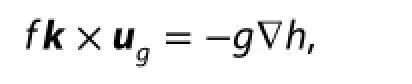
where f is the Coriolis parameter （f（y） = 2ωsin y， in which ω is the rotation rate of the Earth， and y is the latitude）， and g is the gravitational constant.

2.2. SOM analysis

SOM analysis is a dimension-reducing and visualization technique used to map high-dimensional data to a lowdimensional feld. It performs a nonlinear projection from sample vectors to a set of SOM units， for feature extraction and clustering， and each unit has a weight vector （Liu，Weisberg， and Mooers 2006）.

The neural network is composed of an input and output layer. The input layer corresponds to the sample vectors

where n is the sample number and s is the sample size. The output layer is composed of the weight vector array with m being the number of SOM units. The size of the weight vectorwjis equal to the sample size. For the sample vectorxi， the weight vector wj（j=1，2，...，m）showing the minimum Euclidian distance ciis selected as the ‘winner'（or best matching unit， BMU）， which is most similar to the sample vectorxi. This function is expressed as

Furthermore， the training process may update the winner weight vectors by a certain competitive learning rule. This learning rule can be shown aswhere t denotes the current training iteration， xirepresents the input sample vector， α（t） represents a time-decreasing learning rate， and μ（t） is a spatiotemporal neighborhood function， which connects the weight vector with its adjacent weight vector. The radius of the neighborhood may decrease during the training process.

Typically， two evaluation criteria are used for the quality of the SOM: the mean quantization error （QE） and topographic error （TE）. QE is the average distance between each sample vector and its BMU， which be used to measure the map resolution. TE is the proportion of all sample vectors for which frst and second BMUs are not adjacent units，which can be used to evaluate the topology preservation. The minimum QE indicates the most accurate representation of the input data， while the minimum TE indicates the best SOM pattern organization such that adjacent to a BMU in the map lattice is the second BMU （Liu， Weisberg，and Mooers 2006）.

Despite its wide range of applications as a tool for feature extraction and clustering， in SOM analysis the choice of parameters remains a challenge， because diferent parameter choices may result in diferent SOM units. Hence， sensitivity studies have been performed to ascertain the efects of tunable SOM parameters （Liu， Weisberg， and Mooers 2006）. In this paper， we choose suitable parameter settings according to the results of their study， such as a rectangular lattice for small map sizes， a ‘sheet' map shape， linearly initialized weights， and an ‘ep' neighborhood function with initial and fnal neighborhood radii of 1 and 1. On the other hand， we also compare the results based on diferent map sizes （2 × 2， 2 × 3， and 3 × 4）. The results show that the larger map size results in smaller QE and larger TE. In addition， we fnd that most of the SOM units obtained using the larger map size can be further classifed into three types，which are similar to the units based on the 2 × 2 map size. Moreover， most studies focus on the low-frequency variations， such as the decadal modulation between two states（e.g. Qiu and Chen 2010）. Thus， the smaller map size of 2 × 2 is further used. Finally， the batch training is performed over 50 iterations， so that the fnal QE and TE are stable.

3. Results

To investigate the characteristics of the SLA in the KE region from January 1993 to December 2014， the area covering （29.875—40.125°N， 139.875—160.125°E） is chosen to perform the SOM analysis. Here， the main focus is on the low-frequency variations.

3.1. Climatic characteristics of the SLA

Figure 1.（a） Climatological mean sea level felds from January 1993 to December 2014， based on the AVISO gridded data-set. Black contours denote the mean SSH （units: m）， with a contour interval of 0.1 m. Color shading denotes the meridional SSH gradient. The path of the KE jet， defned by the 100-cm contour，is shown in bold. （b） Standard deviation （units: m） of the monthly mean SSH signals for the period January 1993 to December 2014. （c） Time series of the monthly SLA data （units: m） averaged over the region （30—40°N， 140—160°E）. The red line denotes the 13-month moving average.

In general， the path （or axis） of a quasi-geostrophic current is considered as the location of its maximum meridional surface height gradient∂h/∂y， as well as its maximum zonal surface velocity. From the long-term mean SSH feld（Figure 1（a）； equally applicable to the monthly data）， the 100-cm contour is consistently located at， or near， the maximum height gradient， and thus may be a good indicator of the KE jet path. Hence， we choose the 100-cm contour to represent the KE path in the present study.

As shown in Figure 1（a）， in the upstream KE region （32—38°N， 141—154°）， the KE path is found nearly zonally in the latitude band 34—36°N， and characterized by the presence of quasi-stationary meanders with two ridges at 144°E and 149°E. Meanwhile， the whole KE region presents a large amplitude of the SSH anomaly， particularly the upstream region （Figure 1（b））. Secondly， as can be seen from the timeseries of the SLA in Figure 1（c）， for a 13-month moving average， the sea level fuctuation shows signifcant interannual modulation， with positive SLAs during 1993—1994，1999—2004， and 2010—2012， and negative anomalies during 1996—1998 and 2006—2009.

On the other hand， previous studies have also detected a complex mesoscale variability （i.e. mesoscale cyclonic/ anticyclonic SLAs）， which causes the KE system to undergo a clearly defned decadal modulation through eddy—mean fow interaction （Qiu and Chen 2010）. Thus， it is meaningful to obtain the main spatial structures of SLAs， as well as their decadal evolution.

3.2. Characteristic patterns

After performing the SOM analysis， we are able to obtain four spatial classifcation patterns of SLA （Figure 2）， where each pattern represents a characteristic structure. The occurrence frequency of each pattern is also marked on each map. Note that the KE paths （purple lines in Figure 2）and sea surface velocities （Figure 3） are both composites based on the time series of the BMU （detailed in Section 3.3）. Figure 2 shows that SOM1， which has an occurrence frequency of 33%， exhibits a wave train structure shown as ‘positive （34°N， 145°E）—negative （36°N， 147°E）—positive（35°N， 150°E）' anomalies in the upstream KE area. Two positive anomalies are located in the south of the ridge， and a negative one between positive anomalies located in the north of the trough. It reveals an anticyclonic forcing in the ridge and a cyclonic forcing in the trough， of the KE's quasi-stationary meanders. For this structure， the KE path is similar to the mean state， and has a large SSH gradient along the KE path. These can all lead to a narrow and strong KE jet that maintains a stable and weakly meandering state （Figure 3）.

Figure 2.Composites for the SOM patterns based on the BMU time series.

SOM2， with an occurrence frequency of 28%， also presents a wave train structure， shown as ‘negative （35°N，145°E）—positive （37°N， 148°E）—negative （35°N， 151°E）' anomalies. Superimposed on the mean KE path， one can see that this pattern causes the quasi-stationary meanders to move to the southwest， and the trough and ridge tend to deepen slightly. The KE stream of this pattern in Figure 3 maintains a single path with a wider meridional amplitude （i.e. larger meridional width） and weaker fow velocity， which is consistent with the weakening of the southern recirculation gyre.

SOM3 has an occurrence frequency of 24%. The spatial pattern exhibits two tripole structures， shown as ‘negative—positive—negative' anomalies. The frst one is north—south oriented and located near 144°E， and the second is northeast—southwest oriented and located near the downstream of the eastern ridge. Positive anomalies of these two structures are distributed along the KE path. These all cause the path move to the northeast. Meanwhile， as shown by the composite geostrophic velocity in Figure 3，the western tripole structure causes a strong meandering fow near 36°N and a slight branch in the region （32—33°N，142—146°E）.

SOM4， which has an occurrence frequency of 15%， is characterized by a strong north—south dipole structure located at 144°E， with a positive value in the north and a negative value in the south. Superimposed on the mean KE path， this dipole causes ridge deepening in the north， and then deepening of the adjacent trough in the south. The path of this pattern is unstable and longer. On the other hand， the surface fow coincident with SOM4 （Figure 3），has a strong double-branch jet structure. Conversely， compared with SOM3， the fow of SOM4 is weak and exhibits a strong splitting. In fact， this dipole structure is similar to blocking in the atmosphere. Previous studies have indicated that the blocking can divide the fow into double branches. Similarly， SOM4 may represent a typical double-branch structure.

Figure 3.Maps of the sea surface fow for the SOM patterns in Figure 2.

In addition， as is well known， the KE system exhibits clearly defned decadal modulation. Qiu et al. （2014）constructed a time series of the SSH anomalies averaged within （31—36°N， 140—165°E）， to indicate this modulation（Qiu et al. 2014； Figure 4）. Here， we defne a dynamic state with SSH anomalies equal to or greater （less） than +5 （-5）cm as a stable （unstable） state. There are six （2002， 2003，2004， 2010， 2011， and 2012） stable and six （1995， 1996，1997， 2006， 2007， and 2008） unstable states based on the above classifcation. In Figure 4， the composite SLA feld for the stable （unstable） state is similar to the spatial pattern of SOM1 （SOM2）. On the other hand， the occurrence of SOM1 （SOM2） is roughly consistent with the stable （unstable） state （Figure 5； detailed in Section 3.3）. Therefore， we consider that the SOM analysis can capture similar patterns for the two states of the KE system.

Figure 4.Composites for two dynamic states of the KE system based on SSH anomaly signals.

To compare， we also perform an EOF analysis of the same SLA data. The percentages of the variance of each EOF mode are 12%， 8%， 6%， and 5%， respectively， and the cumulative percentage is just 31%. Firstly， the results shown in Figure 6 indicate that the EOF1 spatial pattern is similar to SOM1， and EOF2 is similar to SOM4. The SOM analysis can also capture the main patterns extracted by the EOF method. Secondly， for the stable and unstable states of the KE system， the two composites of SLA tend to present a nonlinear relationship （i.e. SOM1 and SOM2）. The position and intensity of the SLA extreme centers are asymmetric under diferent states， which are symmetric in diferent phases of EOF1. Thirdly， it is identifed by the SOM analysis， and not by the EOF method， that the nonlinear patterns （i.e. SOM2 and SOM3） of SLA are associated withthe noticeable south—north movement of the KE path. This movement has also been discussed in previous studies（Qiu and Chen 2005， 2010）. Hence， the main EOF modes are not better at refecting the long-term SLA changes；SOM analysis is more accurate and intuitive.

Figure 5.Time series of the BMU from January 1993 to December 2014.

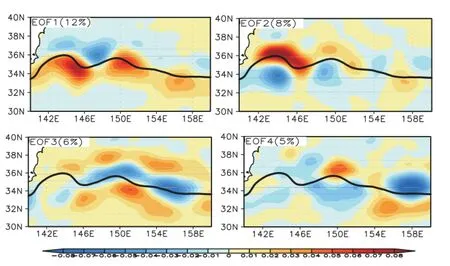
Figure 6.Spatial patterns of the SLA felds （color shading； units: m） based on EOF analysis.

3.3. Time series of the BMU

For each sample of input data， a BMU is defned by the unit that has the smallest weighted distance from the sample data. The BMU time series can refect the evolution of these patterns. In this study， it is useful to examine the temporal changes of the SLA spatial distribution through the use of the BMU time series.

To examine the interannual variations of the SLA， a map of the time series is constructed， as shown in Figure 5. From this fgure， it is apparent that a dominant unit can be identifed for most years. SOM1 mainly happens in 1993—1994，2002—2004， and 2011. SOM2 mainly appears during the years of 1996， 1998， and 2006—2009. In addition， SOM3 emerges in 2000， 2012， and 2014， while SOM4 is apparent in 1999， 2001， and 2013.

On the other hand， combined with the corresponding surface velocity of SOM patterns shown in Figure 3， one can see that the four SOM patterns have a very close relationship with the KE stream. In the upstream KE region， SOM1 and SOM2 represent a single-branch jet structure as the positive phase of the Kuroshio Extension dipole （KED） mode does （Luo， Feng， and Wu 2016）， while SOM3 and SOM4 represent a double-branch jet structure. Thus， the variation of the KE jet structure has a clear decadal period， which can also be seen from the yearly geostrophic velocity felds.

4. Discussion and conclusions

In this paper， SOM analysis is used to extract the characteristic patterns of the SLA in the KE region from January 1993 to December 2014， with a particular focus on decadal variation. The key fndings of the study can be summarized as follows:

The SOM method extracts four characteristic spatial patterns of the SLA， each with its own evolution. SOM1 is found to mainly appear in 1993—1994， 2002—2004，and 2011， with a wave train structure shown as ‘positive （34°N， 145°E）—negative （36°N， 147°E）—positive （35°N，150°E）' anomalies alternately located in the trough and ridges， of the upstream KE's quasi-stationary meanders. This structure remains in a stable state， and with a strengthened （narrower and faster） single-branch jet. SOM2 mainly appears in the years 1996， 1998， and 2006—2009. It too represents a zonal wave train structure， presenting an alternate distribution with ‘negative（35°N， 145°E）—positive （37°N， 148°E）—negative （35°N，151°E）' anomalies. This wave train causes the path to move to the southwest， and makes the single-branch jet unstable through widening and weakening. In addition， SOM3 happens in 2000， 2012， and 2014. It exhibits two tripole structures， leading the path to shift to the northeast. The meridional ‘negative—positive—negative' tripole structure， which is located at 144°E， causes a stronger jet and a relatively weaker branch in the south. SOM4 appears in the years 1999， 2001， and 2013. It is characterized by a dipole structure， with positive values in the north and negative values in the south， located at 144°E， which makes the trough and ridge deepen. The path of this pattern may be unstable and longer. Similar to SOM3， there is a weak branch in the south too. The position of the branch in SOM4 is farther north and stronger than that in SOM3. It is the typical pattern of a double-branch structure.

The spatial patterns of SOM1 and SOM2 are mainly found in the years 1993—1998 and 2002—2011， leading to a single zonal fow. However， the spatial patterns of SOM3 and SOM4 are found to be dominant in the years 1999—2001 and 2012—2014， and are accompanied by a double-branch jet. The SLAs exhibit interannual variation，while the jet structure of the upstream KE region shows decadal variation.

Additionally， through comparison with EOF analysis，SOM analysis is found to be able to accurately characterize the SLA patterns， their evolution， and alternation between patterns， during the period 1993—2014. In short，when studying the KE region， SOM analysis is superior to EOF analysis.

Finally， it is important to note that， although the characteristics of the SLA are classifed using the SOM method in this paper， the nonlinear dynamical mechanism of such a classifcation is not investigated. Further study on this topic is needed in future work.

Disclosure statement

No potential confict of interest was reported by the authors.

Funding

This work was supported by the National Basic Research Program of China （973 Program） ［grant number 2013CB956203］.

References

Anny， C.， and L. William. 2010. “Contemporary Sea Level Rise.”Annual Review of Marine Science 2: 145—173. doi:10.1146/ annurev-marine-120308-081105.

Aoki， S.， and S. Imawaki. 1996. “Eddy Activities of the Surface Layer in the Western North Pacifc Detected by Satellite Altimeter and Radiometer.” Journal of Oceanography 52 （4）: 457—474. doi:10.1007/bf02239049.

Ducet， N.， P. Y. L. Traon， and G. Reverdin. 2000. “Global Highresolution Mapping of Ocean Circulation from TOPEX/ Poseidon and ERS-1 and -2.” Journal of Geophysical Research 105 （C8）: 19477—19498. doi:10.1029/2000jc900063.

Ebuchi， N.， and K. Hanawa. 2000. “Mesoscale Eddies Observed by TOLEX-ADCP and TOPEX/POSEIDON Altimeter in the Kuroshio Recirculation Region South of Japan.” Journal of Oceanography 56 （1）: 43—57. doi:10.1023/A:1011110507628. Kelly， K. A.， R. J. Small， R. M. Samelson， B. Qiu， T. M. Joyce，Y.-O. Kwon， and M. F. Cronin. 2010. “Western Boundary Currents and Frontal Air-Sea Interaction: Gulf Stream and Kuroshio Extension.” Journal of Climate 23 （21）: 5644—5667. doi:10.1175/2010jcli3346.1.

Liu， Y.， and R. H. Weisberg. 2007. “Ocean Currents and Sea Surface Heights Estimated across the West Florida Shelf.” Journal of Physical Oceanography 37 （6）: 1697—1713. doi:10.1175/ jpo3083.1.

Liu， Y.， and R. H. Weisberg. 2011. Self Organizing Maps - Applications and Novel Algorithm Design: A Review of Self-organizing Map Applications in Meteorology and Oceanography. Slavka Krautzeka 83/A 51000 Rijeka， Croatia: InTech.

Liu， Y.， R. H. Weisberg， and C. N. K. Mooers. 2006. “Performance Evaluation of the Self-Organizing Map for Feature Extraction.”Journal of Geophysical Research 111 （C05018）: 1—14. doi:10.1029/2005jc003117.

Luo， D.， S. Feng and L. Wu. 2016. “The Eddy-Dipole Mode Interaction and the Decadal Variability of the Kuroshio Extension System.” Ocean Dynamics. doi:10.1007/s10236-016-0991-6.

Pierini， S.， and H. A. Dijkstra. 2009. “Low-frequency Variability of the Kuroshio Extension.” Nonlinear Processes in Geophysics 16（6）: 665—675. doi:10.5194/npg-16-665-2009

Qiu， B.， and S. Chen. 2005. “Variability of the Kuroshio Extension Jet， Recirculation Gyre， and Mesoscale Eddies on Decadal Time Scales.” Journal of Physical Oceanography 35 （11）: 2090—2103. doi:10.1175/jpo2807.1.

Qiu， B.， and S. Chen. 2010. “Eddy-mean Flow Interaction in the Decadally Modulating Kuroshio Extension System.” Deep Sea Research Part II: Topical Studies in Oceanography 57 （13—14）: 1098—1110. doi:10.1016/j.dsr2.2008.11.036.

Qiu， B.， S. Chen， N. Schneider， and B. Taguchi. 2014. “A Coupled Decadal Prediction of the Dynamic State of the Kuroshio Extension System.” Journal of Climate 27 （4）: 1751—1764. doi:10.1175/jcli-d-13-00318.1.

Reusch， D. B.， B. C. Hewitson， and R. B. Alley. 2005. “Towards Ice-Core-Based Synoptic Reconstructions of West Antarctic Climate with Artifcial Neural Networks.” International Journal of Climatology 25 （5）: 581—610. doi:10.1002/joc.1143.

Richardson， A. J.， C. Risien， and F. A. Shillington. 2003. “Using Self-organizing Maps to Identify Patterns in Satellite Imagery.”Progress in Oceanography 59 （2）: 223—239. doi:10.1016/j. pocean.2003.07.006.

Sasaki， Y. N.， S. Minobe， and N. Schneider. 2013. “Decadal Response of the Kuroshio Extension Jet to Rossby Waves: Observation and Thin-Jet Theory*.” Journal of Physical Oceanography 43 （2）: 442—456. doi:10.1175/jpo-d-12-096.1.

Stammer， D.， A. Cazenave， R. M. Ponte， and M. E. Tamisiea. 2013.“Causes for Contemporary Regional Sea Level Changes.”Annual Review of Marine Science 5: 21—46. doi:10.1146/ annurev-marine-121211-172406.

Taguchi， B.， B. Qiu， M. Nonaka， H. Sasaki， S.-P. Xie， and N. Schneider. 2010. “Decadal Variability of the Kuroshio Extension: Mesoscale Eddies and Recirculations.” Ocean Dynamics 60 （3）: 673—691. doi:10.1007/s10236-010-0295-1.

Tatebe， H.， and I. Yasuda. 2001. “Seasonal Axis Migration of the Upstream Kuroshio Extension Associated with Standing Oscillations.” Journal of Geophysical Research 106 （C8）: 16685—16692. doi:10.1029/2000jc000467.

Tracey， K. L.， D. R. Watts， K. A. Donohue， and H. Ichikawa. 2012.“Propagation of Kuroshio Extension Meanders between 143° and 149°E.” Journal of Physical Oceanography 42 （4）: 581—601. doi:10.1175/jpo-d-11-0138.1.

海面异常； 自组织映射分析； 自组织映射模态； 急流变化

27 February 2016

CONTACT LUO De-Hai ldh@mail.iap.ac.cn

© 2016 The Author（s）. Published by Informa UK Limited， trading as Taylor & Francis Group.

This is an Open Access article distributed under the terms of the Creative Commons Attribution License （http://creativecommons.org/licenses/by/4.0/）， which permits unrestricted use， distribution， and reproduction in any medium， provided the original work is properly cited.