
Coherence estimation algorithm using Kendall’s concordance measurement on seismic data*
2016-12-02 07:25YangTaoGaoJingHuaiZhangBingandWangDaXing
Applied Geophysics 2016年3期
Yang Tao, Gao Jing-Huai♦, Zhang Bing, and Wang Da-Xing
Coherence estimation algorithm using Kendall’s concordance measurement on seismic data*
Yang Tao1,2, Gao Jing-Huai♦1,2, Zhang Bing1,2, and Wang Da-Xing3
The coherence method is always used to describe the discontinuity and heterogeneity of seismic data. In traditional coherence methods, a linear correlation coefficient is always used to measure the relationship between two random variables (i.e., between two seismic traces). However, mathematically speaking, a linear correlation coefficient cannot be applied to describe nonlinear relationships between variables. In order to overcome this limitation of liner correlation coefficient. We proposed an improved concordance measurement algorithm based on Kendall’s tau. That mainly concern the sensitivity of the liner correlation coefficient and concordance measurements on the waveform. Using two designed numerical models tests sensitivity of waveform similarity affected by these two factors. The analysis of both the numerical model results and real seismic data processing suggest that the proposed method, combining information divergence measurement, can not only precisely characterize the variations of waveform and the heterogeneity of an underground geological body, but also does so with high resolution. In addition, we verified its effectiveness by the actual application of real seismic data from the north of China.
Concordance measurement, coherence estimation, nonlinear correlation, information divergence
Introduction
The coherence analysis of seismic data, a powerful technique for interpreting seismic data, can clearly describe the faults and lateral changes in lithology (i.e., heterogeneity). Moreover, it improves the efficiency of seismic interpretation. This technique has been widely used in petroleum exploration and development (Chopra and Marfurt, 2007). The first coherence algorithm (denoted as C1) (Bahorich and Farmer, 1995) uses the cross-correlation coefficients of seismic traces in the inline and crossline directions to estimate coherence. Because only three traces are used, this algorithm is efficient and easily executed. However, its anti-noise performance is unsatisfactory. The second-generation coherence algorithm (C2) uses semblance as a coherence estimation (Marfurt et al., 1998), begins by using more seismic trace data to calculate and analyze the coherent value, is fairly stable, and can be applied toseismic data with a low signal-to-noise ratio (SNR). In addition, the SNR and resolution of its seismic coherence data can be improved by adjusting the size of the time window. However, its lateral resolution is low. The third-generation coherence algorithm (C3) is based on eigenstructure decomposition (Gersztenkorn and Marfurt, 1999) and on the eigenstructure of the covariance matrix formed from the traces in the analysis cube. To characterize the coherence value, this method first constructs a matrix of all the seismic traces within a time window, calculates the data covariance matrix, and then defines the coherent value as the ratio of the eigenvalue of the covariance matrix and the trace of the covariance matrix. The C3 algorithm is theoretically superior to the C2 and C1 algorithms because it has antinoise performance, higher lateral resolution, and can detect fracture characteristics and discontinuity (Marfurt et al., 1999). Cohen and Coifman proposed a method for estimating seismic local structural entropy (LSE) as a coherence measurement (Cohen and Coifman, 2002). Lu et al. (2005) developed a coherence estimation algorithm based on higher-order statistics and super traces (Lu et al., 2005), and Li et al. (2006) proposed a dip-scanning coherence algorithm that uses eigenstructure analysis and a super-trace technique to improve the quality of the coherence image (Li et al., 2006). Wang and Lu proposed a coherence enhancement method that applies local histogram specification (LHS) techniques to enhance subtle faults or fractures in coherence cubes, and this method noticeably enhances the details of subtle faults and fractures (Wang and Lu, 2010). Dou et al. proposed a fracture enhancement method combined with histogram equalization, which can also improve fracture cognition and accuracy (Dou et al., 2014). Wang et al. (2015) improved the coherence algorithm with robust local slope estimation (Wang et al., 2015). Many other scholars have also put forward a variety of coherence methods.
Coherence algorithms are primarily based on the measurement of similarity between waveforms or traces (Chopra and Marfurt, 2007). In seismic data interpretation, if the seismic signal is used to observe random variables, there are many possible relationships between these variables and linear correlation is just one of them. While linear correlation between seismic traces can be used to depict subtle changes of seismic waveforms, its precision cannot meet the requirements of seismic interpretation. To address this problem, we propose a coherence algorithm based on Kendall’s tau for seismic data, which emphasizes studying the sensitivity characteristics of waveform change, which is characterized by the correlation measures of seismic wavelets or seismic records. In doing so, this information divergence coherence measurement improves computational efficiency. Finally, we use the improved method to finely depict the boundary of the subsurface geology and the lateral variation of the stratum in processing real seismic data from the north of China.
Coherence algorithm based on Kendall’s concordance measurement
Definition of Kendall measurement
Informally, Kendall’s tau is used to quantitatively characterize the concordance and association of a pair of random variables (Kendall, 1938; Kruskal, 1958; Lehmann and D’Abrera, 1975). Thus, in the fields of mathematics and statistics, the concordance or consistency of two random variables is expressed as follows:
Let (xi, yi) and (xj, yj) denote two observations from a vector (X, Y) of continuous random variables. We say that (xi, yi) and (xj, yj) are concordant if xi< xjand yi< yj, or if xi> xjand yi> yj. Similarly, we say that (xi, yi) and (xj, yj) are discordant if xi> xjand yi> yjor if xi> xjand yi< yj. This can also be equivalently expressed as follows: if (xi– xj)(yi– yj) > 0, (xi, yi) and (xj, yj) are concordant; if (xi–xj)(yi– yj) < 0, (xi, yi) and (xj, yj) are discordant.
Let {(xi, yi), (x2, y2), …, (xn, yn)} denote a random sample of n observations from a vector (X, Y) of continuous random variables, then the Kendall’s tau is expressed as follows (Nelsen, 1999):
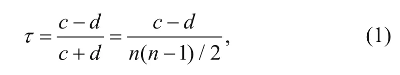
where c denotes the number of concordant pairs, d denotes the number of discordant pairs, and n denotes the number of the sample.
In order to easily understand equation (1), let there be two variables, X = [1, 2, 3] and Y = [4, 3, 5], where n = 3. To measure the concordance, there are n(n–1)/2 pairs in X with Y, and we compare the concordant pairs by the first pairs [4,3] of Y (the value from large to small) corresponding to the first pairs [1,2] of X (the value from small to large), with the c being odd +1. Conversely, to measure discordant pairs, the d is odd +1, and we compute all the pairs in this way with the totalnumber being c – d. Taking c, d, and n into equation (1) as τ, the Kendall’s tau is defined as the probability of concordance or discordance (Nelsen, 1999):

where Pr denotes the probability density function of the variables.
In fact, Kendall provided a method for computing concordance (Kendall, 1938), which is equivalent to the following:

where n denotes the number of sample time points and sign is the sign function.
Comparison of concordance and linear correlation measurements
We designed two models to test the advantages of our proposed method.
Model 1: Assumes that there is a Ricker wavelet, and compares the difference in waveform similarity between the Ricker wavelet and the after-phase rotation of the wavelet, where wois the Ricker wavelet shown in Figure 1a, ||w0|| = 1, w0His the Hilbert transform of wo, and we then obtain the new wavelet wθby rotating phase θ (Levyand Oldenburg, 1987), as shown in equation (4):
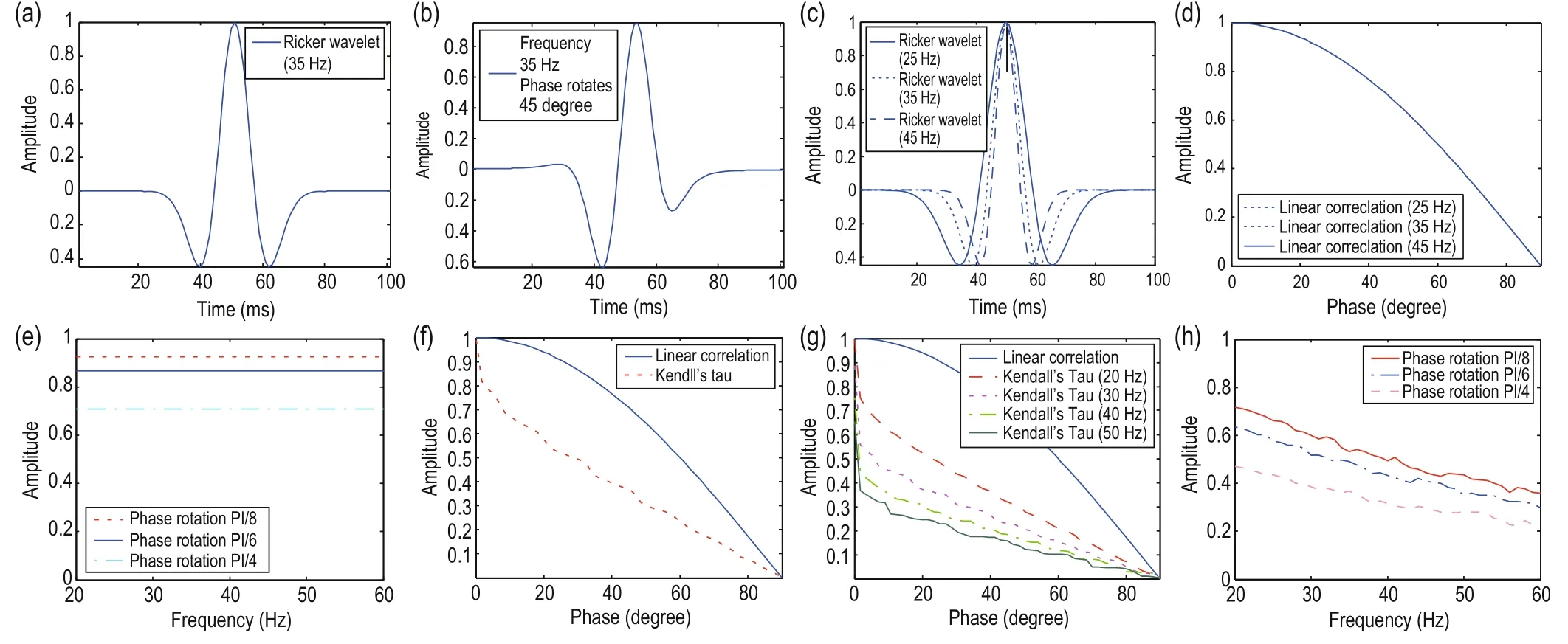
Fig.1 Curves of Ricker wavelet and similarity measurement.

In order to express this more conveniently, let fmdenote the dominant frequency of the wavelet and wθfm denote the wavelet after phase rotation θ. Figure 1c shows wavelets with different dominant frequencies, where the curve cov(w0fm, wθfm) represents the linear correlation between the original wavelet and the wavelet after phase rotation when the dominant frequency of the wavelet is fixed, as shown in Figure 1d. Under the same conditions, the curves completely overlap when fmis different. The correlation coefficient measures can’t describe the waveform similarity caused by the dominant frequency when the wavelet rotates at the same angle. It is easy to prove that cov(w0fm, wθfm) is as follows:

We know from equation (5) that, under the condition of ||w0|| = 1 in this model, the correlation coefficient only describes the variation of waveform similarity caused by phase rotation. This results in concordance, as shown in Figure 1d. In order to further analyze the relationship between the correlation coefficient and the waveform changes caused by dominant frequency or same–phase rotation (choosing the range of the dominant frequency as 20 Hz to 60 Hz and three rotation angles of π/8, π/6, and π/4, respectively), in the measurement curves of waveform variation shown in Figure 1e we can see that the correlation coefficient values are the same even as the frequency gradually increases from 20 Hz to 60 Hz. Therefore, this result verifies that the correlation coefficient cannot describe the similarity change caused by the frequency.
We can obtain the tau measurement curve by applying model 1, as shown in Figure 1f. In addition, to compare the variation of waveform similarity, we chose three different dominant frequencies (25 Hz, 35 Hz, and 45 Hz) to compute the two values. Figure 1g shows the calculation results with phase rotation (from 0 degrees to 90 degrees) in which the curves overlap for the correlation coefficient (solid line) and do not overlap for the tau measurement (dashed line). The tau slope value gradually decreases with decreases in the phase rotation angle, so it demonstrates better sensitivity to waveform change than linear correlation measurement. However, the latter has an advantage over the former when the phase rotation angle is large. The tau measure not only describes the waveform similarity variation caused by phase rotation, but also the waveform similarity variation caused by the dominant frequency. In Figure 1h, with a fixed rotation angle, the tau value gradually decreases with gradual changes in the dominant frequency. We can see that the variation of this curve is smaller, so we consider that tau measurement can better describe waveform similarity variation than linear correlation (due to dominant frequency and phase rotation). When applied to real seismic data, it may describe geological discontinuity and heterogeneity of sand bodies and their characteristics. According to wave theory, it is generally known that there is a change in phase and frequency arising from the wave attenuation and dispersion effect when seismic waves propagate in viscoelastic media.To compare the difference in sensitivity of the tau and linear correlation measurements, we investigated their differences in sensitivity to analyze waveform changes in wavelets in a viscoelastic medium.
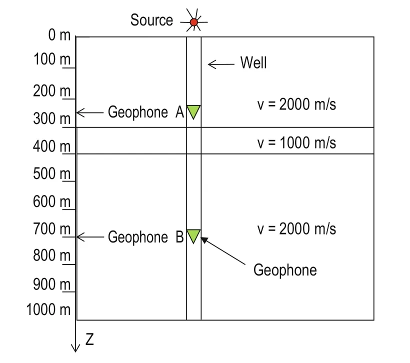
Fig.2 Schematic of stratum model
Model 2: There are three media layers, in which the first and third are elastic media, with a wave velocity (Vp) of υ = 2000 m/s and the second is a diffusive-viscous medium with a Vpof υ = 1000 m/s. The total thickness of the three layers is 1000 m, with the thickness of the first layer being 300 m, of the second 100 m, and of the third 600 m. The second layer’s attenuation factor Q (Zhao et al., 2014) is as follows:

where υ denotes wave velocity, ω denotes the frequency, and γ and η denote diffusive and viscous attenuation parameters, respectively (γ = 20, η = 0.02 here).
The second layer’s velocity is lower than that of the first and third. As shown in Figure 2, we installed a geophone in the well, with the source at the wellhead, and the seismic wavelet is the vertically incident plane wave. Due to the influence of absorption and attenuation on the second layer, the phase, amplitude, and frequency of the wavelet changed. As shown in Figure 4, we placed geophones A and B at depths of 250 m and 700 m in the well, respectively. To compare the sensitivities of the waveform changes, we used the linear correlation and tau measurement to investigate the received signal from geophones A and B. Figure 3 shows the seismic forward record of the vertical seismic profile (VSP), based on the model in Figure 2.
In Figure 2, z denotes the layer depth direction and z = 0 indicates the wellhead. Figures 4a and 4b show the received seismic signals from geophones A and B,respectively. We can take into account only the first breaks of downward moving waves at depths of z = 250 m and z = 700 m, as marked by the elliptical circles in Figure 4. Using these two measurements to describe the variation of waveform similarity in the synthetic seismograms (VSP data), we can observe a seismic wavelet at a depth of 250 m in Figure 5a (marked by w) and geophone B receives signals, as shown in Figures 5b and 5a, at depths of z = 400 m and z = 500 m, respectively.
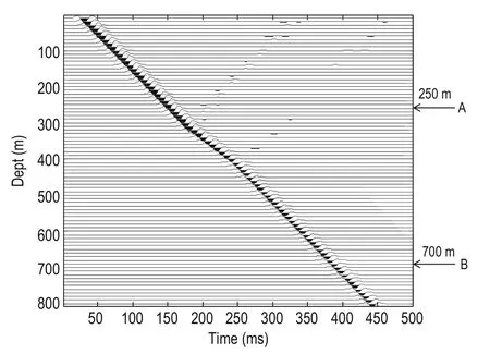
Fig.3 Synthetic seismogram of zero-offset VSP data

Fig.4 Seismic records received by geophones A and B at depths of 250 m and 700 m, respectively.
To describe small changes in waveform, we fixed the top interface of the second layer, and slowly lowered the lower interface to add thickness and receive downward waves by geophone B that correspond to each change in thickness. Specifically, we fixed the top interface at z = 300 m and lowered the lower interface from z = 400 m to z = 500 m, with Δz = 10 m. Figures 5a and 5b show the effect of absorption and attenuation on waveform change for wavelets at z = 400 m and z = 500 m, respectively. Due to the absorption and attenuation of the middle layer, the waveform changed as marked at positions a and b. The measurement result between w and wBkis shown in Figure 5d by the linear correlation and tau measure, respectively, and wBkis the received downward wave by geophone B when the thickness of the second layer is 100 + kΔz (1 ≤ k ≤ 10). We can see from Figure 5d that the tau measurement curve has a greater change than the linear correlation curve for a thickness interval of 10 m. When the thickness is less than 170 m, the tau measurement is more sensitive to variation in waveform. In Figure 5d we see that h1 is the difference value of waveform similarity derived from the linear correlation measure and h2 is that from the tau measure, but the thickness is greater than 170 m (the two measurement curves have same trend with increasing thickness in Figure 5d, with the upward end of the curve arising from curve fitting).
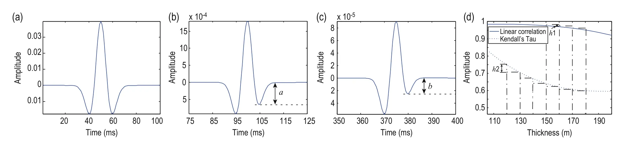
Fig.5 Seismic wavelets at different depths and waveform similarity curves for different thicknesses.
A comparison of the results of the two models clearly shows that tau measurement can describe small waveform change for larger phase rotations such as those found in faults, fissures, and channels, and this trend coincides with both measurements. For larger changes in geological structure, a description of geological structure can be easily achieved using the traditional methods, but to describe the local information of complex geological structures, a new method is required. If we apply tau measurement to process real seismic data, we may be able to increase the resolution for describing anisotropies and discontinuities. As such, here we propose a coherence analysis method based on many seismic traces using tau measurement (denoted as D-tau).
D-tau coherence algorithm
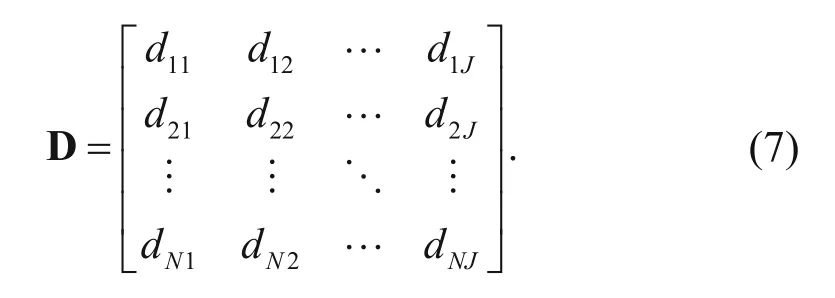
For 3D seismic data, let wIand wcbe analysis windows in the crossline and inline directions, respectively, where wTis the number of time samples, which form a subvolume. The combination of the seismic trace target(marked as 5) and its adjacent seismic traces is shown in Figure 6. We compute the tau measurement between the central and adjacent traces as in the analysis method for the coherent data volume. Let NI× NC= J, for which wIhas NItraces and wchas NCtraces, and wThas NTsample points. The sizes of the analysis window rectangle A, as shown in Figure 6, is NI= 3, NC= 3 and NT= N. According to the marked position label, we order all the traces in the analysis window with respect to the data matrix D (N line and J column). dijdenotes the ith row and jth column, and when the central trace moves to marking 5' or 5", the position of the analysis window moves in the crossline and inline directions, respectively, as shown in rectangles B and C in Figure 6.
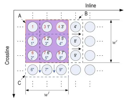
Fig.6 Schematic diagram of the selection of many seismic traces.
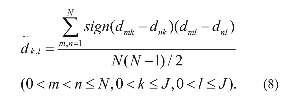
Each column of the matrix denotes a trace within the analysis window. To facilitate the calculation of tau measurement between traces, let variables k and l represent the number of traces, which are taken into equation (3), and are shown as equation (8) below:
We can obtain a semi-definite matrix C by computing the tau measurement between the traces (for all k and l, k, l = 1, …, J).
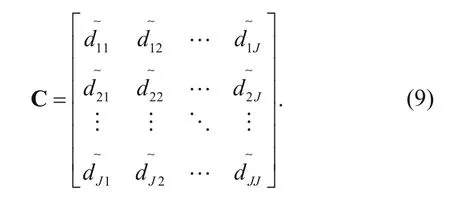
In the C3 algorithm, we perform eigenvalue decomposition of the covariance matrix and then use the eigenvalues to analyze the coherence of the seismic data. Here we use the tau measurement as an extension of the linear correlation, and use matrix C to describe the geological structure.
A large amount of calculation is required to directly calculate matrix eigenvalues, and we use the coherence method based on information divergence without calculating the eigenvalues, which greatly increased the calculation speed while maintaining precision (Yang et al., 2013). This method uses the Rényi divergence coherence measurement and its mathematical expression is as follows (Yang et al., 2013):
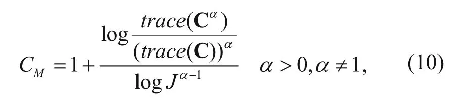
In equation (10), J is the dimension of the matrix; trace(·) is the trace of the matrix; α is a parameter of Rényi information divergence (Rényi, 1959, 1961; Salicrú, 1994), and α is used to adjust the precision of the coherence measurement. In order to achieve computation efficiency by this method, we select the parameter α = 2. CMis the tau measurement of the target point within the analysis window, and we can obtain the 3D seismic coherence data by equation (10) to compute the value of the tau measurement on all the analysis points. In summary, Figure 7 shows a calculation step flow diagram of our proposed concordance measurement method based on Kendall’s tau measurement for seismic data analysis.
Example of real seismic data
To validate the effectiveness of our proposed method, we used the C3 algorithm and D-tau algorithm to estimate real seismic data with the same conditions and compared their results. We obtained real seismic data from the nor2Ah of China, in which there are 650 inlines and 850 crosslines, with each trace having 301 sampling points, intervals of 25 m, and 2-ms sampling rate. The target layer of the seismic data in north China is represented by the box H8 reservoir, with an average porosity of 8.8%, average permeability of 0.732 D, sandbody thickness ranging from 10 m-40 m, and layer thickness ranging from 3 m-10 m. The sand body is vertically superimposed and transversely contiguous and has strong heterogeneity. The gas reservoir is thin and scattered and has poor connectivity, is not controlledby the structure, and is a typical low-permeability gas reservoir.
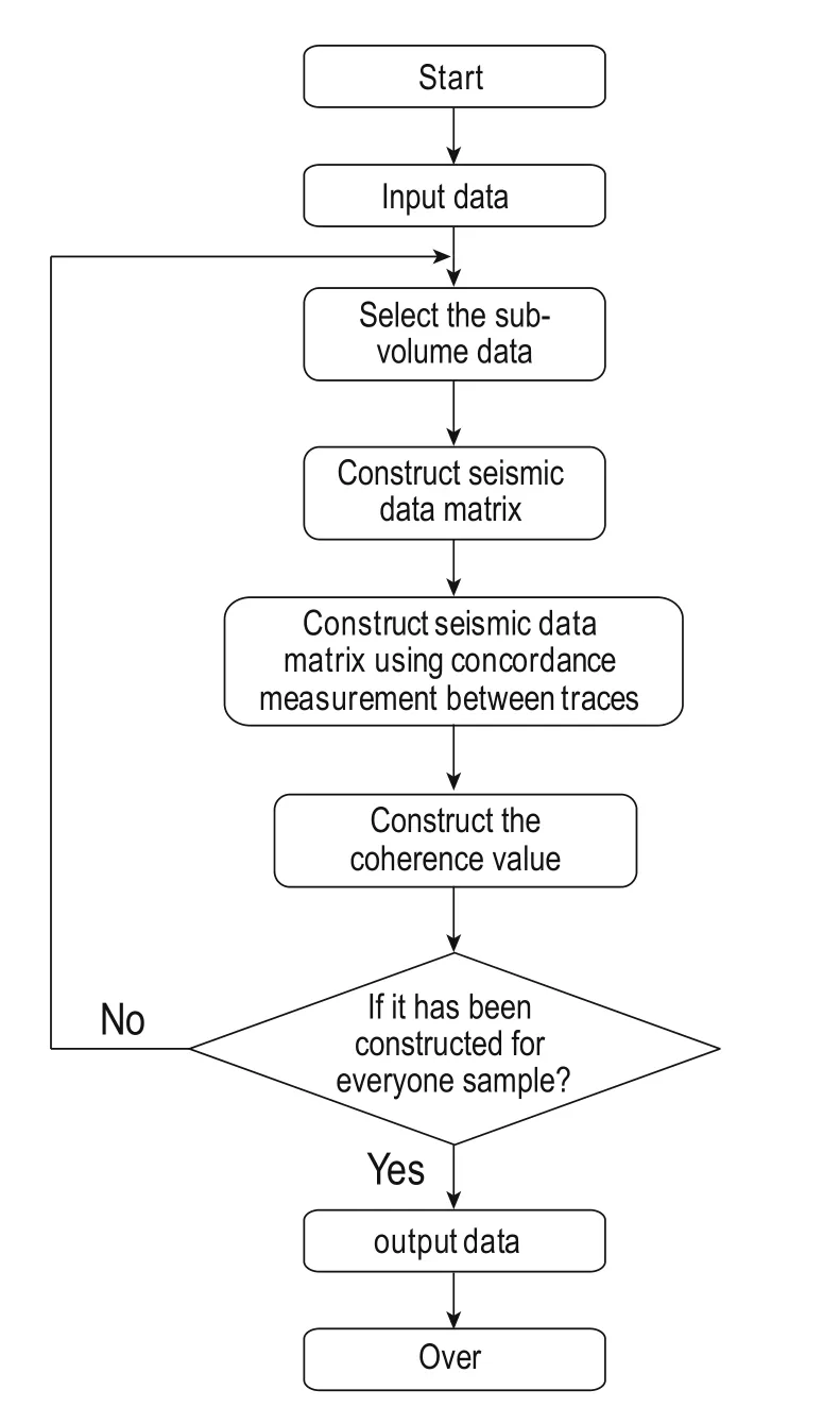
Fig.7 Flow diagram of the concordance measurement method.

Fig.9 Coherence horizon slices.
In this study, we used the D-tau algorithm and C3 algorithm in MAIS software to estimate the coherence data obtained by the flow diagram (Figure 7), respectively. To initialize the parameters of the analysis window, including the window size and time sample points, we did not consider the effect of azimuth and dip because the strata are almost horizontal, and the azimuth and dip are small when we estimate the coherence data in the work area. Next, we loaded the data, determined the target points, selected the sub-volume, constructed the covariance matrix (as in equation (7)), and calculated the concordance and coherence values using equation (10) toobtain the coherence data for every target point. In order to conveniently compare the two coherence methods, we marked the selected sand bodies with a black circle. The original seismic data horizon slice is shown in Figure 8, and the coherence volumes estimated using the C3 and D-tau algorithms correspond to Figures 9a and 9b, respectively.

Fig.8 Original seismic data horizon slice.
From Figure 9, we can see that the D-tau algorithm clearly depicts the edge of the sandstone reservoirs (marked by black circles) and the heterogeneity (marked by arrows) (Figure 9a), but the C3 algorithm coherence slices show only a vague edge of the sand body and vague heterogeneity (Figure 9a). That said, Figure 9b is more in line with the actual geological conditions. In order to further test and verify the D-tau algorithm, we selected one profile from the crossline direction of the original data (Figure 10a), which corresponds to the black lines marked in Figures 8 and 9. Figures 10b and 10c show the coherence profiles of the C3 algorithm and the D-tau algorithm, respectively. We can see that the coherence profiles of the D-tau algorithm clearly describe the edge position of the sand body and enhance the weak coherence information, compared to the C3 algorithm results.
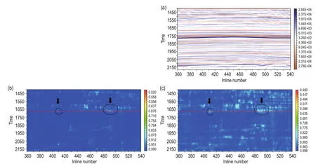
Fig.10 Profiles in the crossline direction.
In addition, we selected one profile from the inline direction, as shown in Figure 11. Figure 11a shows the original seismic profile in which there is some event pinched out, as marked by the circles, and some smaller faults marked by the rectangles. Figures 11b and 11c show the coherence profiles of the C3 and D-tau algorithms, respectively. From the two figures, we can see that that the C3 algorithm is weaker in describing the geological characteristics. The D-tau algorithmmore clearly depicts the geological features and better describes the reservoir heterogeneity with few changes in the stratigraphic structure of the coherence profile.

Fig.11 Profiles in the inline direction.
Conclusions
In this paper, we proposed an improved coherence algorithm (D-tau) based on Kendall’s tau. The emphasis of which is to study the sensitivity of linear correlation measurement and concordance measurement on the variation of seismic waveform. We introduce Kendall’s concordance measurement, which extends the linear correlation to include nonlinear correction concordance, and can capture dependent interrelationships between seismic traces. The two models were designed with changing of the phase and dominant frequency of wavelet and attenuation, absorption of wavelet based on wave theory, and were used to test the sensitivity of the different measurements, By comparison, tau measurement has much more sensitivity to waveform similarity than linear correlation, which we verified using two models. In addition, our proposed model introduces and integrates existing work by this paper’s authors to apply an information divergence coherence measure for estimating coherence values within an analysis window. Both the model example results and real seismic data processing demonstrate the validity of our proposed approach in characterizing with high resolution the edge of a sand body and the heterogeneity of an underground geological body and its faults. However, this method lacks some calculation efficiency in computing linear correlation with respect to concordance. To address this problem, future research will take into account calculation efficiency and the influencing factors of dip and azimuth.
Acknowledgements
The authors would like to thank all the teachers and students at the Institute of Wave and Information at Xi’an Jiaotong University for their help. We also greatly appreciate the Major Programs of National Natural Science Foundation of China (Grant No. 41390454); the Major Research Plan of the National Natural Science Foundation of China (Grant No. 91330204) for their support, also highly appreciate the Editor-in-chief and reviewers for their constructive comments and suggestions.
Bahorich, M. S., and Farmer, S. L., 1995, 3-D seismic discontinuity for faults and stratigraphic features: The coherence cube: The Leading Edge, 14, 1053-1058.
Chopra, S., and Marfurt, K., 2007, Seismic attributes for prospect identification and reservoir characterization: Society of Exploration Geophysicists Geophysical Developments, 11, Tulsa, Oklahoma.
Cohen, I., and Coifman, R. R., 2002, Local discontinuity measures for 3-D seismic data: Geophysics, 67, 1933-1945.
Dou, X. Y., Han, L. G., Wang, E. L., Dong, X. H., Yang, Q., and Yan, G. H., 2014, A fracture enhancement method based on the histogram equalization of eigenstructurebased coherence: Applied Geophysics, 11, 179-185.
Gersztenkorn, A., and Marfurt, K. J., 1999, Eigenstructurebased coherence computations as an aid to 3-D structural and stratigraphic mapping: Geophysics, 64, 1468-1479.
Kendall, M. G., 1938, A new measure of rank correlation: Biometrika, 30, 81-93.
Kruskal, W. H., 1958, Ordinal Measures of Association: Journal of the American Statistical Association, 53, 814-861.
Lehmann, E. L., and D'Abrera, H. J. M., 1975, Nonparametric statistical methods based on ranks: Journal of the Royal Statistical Society, 83(140), 347-353.
Levy, S., and Oldenburg, D., 1987, Automatic phase correction of common-midpoint stacked data: Geophysics, 52, 51-59.
Li, Y., Lu, W., Zhang, S., and Xiao, H., 2006, Dip-scanning coherence algorithm using eigenstructure analysis and supertrace technique: Geophysics, 71, V61-V66.
Lu, W., Li, Y., Zhang, S., Xiao, H., and Li, Y., 2005, Higher-order-statistics and supertrace-based coherenceestimation algorithm: Geophysics, 70, P13-P18.
Marfurt, K. J., Kirlin, R. L., Farmer, S. L., and Bahorich, M. S., 1998, 3-D seismic attributes using a semblance-based coherency algorithm: Geophysics, 63, 1150-1165.
Marfurt, K. J., Sudhaker, V., Gersztenkorn, A., Crawford, K.D., and Nissen, S.E., 1999, Coherency calculations in the presence of structural dip: Geophysics, 64, 104-111.
Nelsen, R. B., 1999, Lecture Notes in Statistics: Dependence, 3(1), 139-146.
Rényi, A., 1959, On a theorem of P. Erdős and its application in information theory: Mathematica (Cluj), 1(24), 341–344.
Rényi, A., 1961, On measures of entropy and information: in Neyman, J., Ed., Fourth Berkeley Symposium on Mathematical Statistics and Probability: University ofCalifornia Press, Berkeley, 1, 547–561.
Salicrú, M., 1994, Measures of information associated with Csiszar's divergences: Kybernetika Praha, 30(5), 563–573.
Wang, J., and Lu, W. K., 2010, Coherence cube enhancement based on local histogram specification: Applied Geophysics, 7, 249–256.
Wang, Y., Lu, W., and Zhang, P., 2015, An improved coherence algorithm with robust local slope estimation: Journal of Applied Geophysics, 114, 146-157.
Yang, T., Zhang, B., and Gao, J., 2013, A fast coherence algorithm for seismic data interpretation based on information divergence: SEG Technical Program Expanded Abstracts, 2554-2558. Zhao, H., Gao, J., and Liu, F., 2014, Frequency-dependent reflection coefficients in diffusive-viscous media: Geophysics, 79, T143-T155.

Yang Tao Ph.D. graduated at Xi’an Jiaotong University, focusing on seismic signals processing and seismic attributes.
Email: yangtao610@163.com
Manuscript received by the Editor August 15, 2015; revised manuscript received September 9, 2016.
*This work was supported by the Major Programs of National Natural Science Foundation of China (No. 41390454) and the Major Research Plan of the National Natural Science Foundation of China (No. 91330204).
1. Institute of Wave and Information, Xi'an Jiaotong University, Xi’an 710049, China.
2. National Engineering Laboratory for Offshore Oil Exploration, Xi'an 710049, China.
3. Exploration and Development Research Institute of Petrochina Changqing Oil Field Company, Xi'an 710018, China.
♦Corresponding author: Gao Jing-Huai (Email: jhgao@mail.xjtu.edu.cn)
© 2016 The Editorial Department of APPLIED GEOPHYSICS. All rights reserved.

- Applied Geophysics的其它文章
- Spherical cap harmonic analysis of regional magnetic anomalies based on CHAMP satellite data*
- 3D modeling of geological anomalies based on segmentation of multiattribute fusion*
- Three-dimensional numerical modeling of fullspace transient electromagnetic responses of water in goaf*
- 3D finite-difference modeling algorithm and anomaly features of ZTEM*
- Prismatic and full-waveform joint inversion*
- Anomalous astronomical time-latitude residuals: a potential earthquake precursor*