
On the modeling of viscous incompressible flows with smoothed particle hydrodynamics*
2016-12-06 08:15MouBinLIU刘谋斌ShangmingLI李上明
水动力学研究与进展 B辑 2016年5期
Mou-Bin LIU (刘谋斌), Shang-ming LI (李上明)
1. College of Engineering, Peking University, Beijing 100871, China
2. Institute of Ocean Research, Peking University, Beijing 100871, China
3. State Key Laboratory for Turbulence and Complex systems, Peking University, Beijing 100871, China,
4. Institute of Systems Engineering, China Academy of Engineering Physics (CAEP), Mianyang 621900, China
E-mail: mbliu@pku.edu.cn
On the modeling of viscous incompressible flows with smoothed particle hydrodynamics*
Mou-Bin LIU (刘谋斌)1,2,3, Shang-ming LI (李上明)4
1. College of Engineering, Peking University, Beijing 100871, China
2. Institute of Ocean Research, Peking University, Beijing 100871, China
3. State Key Laboratory for Turbulence and Complex systems, Peking University, Beijing 100871, China,
4. Institute of Systems Engineering, China Academy of Engineering Physics (CAEP), Mianyang 621900, China
Smoothed particle hydrodynamics (SPH) is a Lagrangian, meshfree particle method and has been widely applied to different areas in engineering and science. Since its original extension to modeling free surface flows by Monaghan in 1994, SPH has been gradually developed into an attractive approach for modeling viscous incompressible fluid flows. This paper presents an overview on the recent progresses of SPH in modeling viscous incompressible flows in four major aspects which are closely related to the computational accuracy of SPH simulations. The advantages and disadvantages of different SPH particle approximation schemes, pressure field solution approaches, solid boundary treatment algorithms and particle adapting algorithms are described and analyzed. Some new perspectives and future trends in SPH modeling of viscous incompressible flows are discussed.
smoothed particle hydrodynamics (SPH), viscous incompressible flow, free surface flow, fluid-structure interaction(FSI)
Introduction
Viscous incompressible flows in ocean and coastal hydrodynamics and offshore engineering are significantly important as they can greatly influence the nearly personnel and structures. Typical viscous incompressible flow phenomena include wave dynamics(waver generation, wave breaking, and wave interaction with other structures), dam breaking, water filling and water discharge (to and from a water tank or reservoir), shallow water flows, entry and exit of water,sloshing phenomena with fluid-solid interaction, and many different other problems. These flow phenomena involve special features, which are difficult for numerical simulation. For example, viscous incompressible free surface flows with moving objects involve rapid movement of solid objects, change and breakup of free surfaces, strong turbulence and vortices, and violent fluid-solid interaction. The tremendous hydro-pressure load can cause neighboring structures to deform elastically or even plastically.
For modeling viscous incompressible flows, the grid-based numerical methods such as finite difference method (FDM), finite volume method (FVM) and Finite Element method (FEM) are the most frequently used approaches. So far the grid-based numerical models have achieved remarkably, and they are currently the dominant methods in computational fluid dynamics (CFD) or computational solid dynamics(CSD). Despite the great success, grid-based numerical methods suffer from difficulties, which limit their applications in modeling viscous incompressible flows such as hydro-elastic problems with violent deformation and even break up of free surfaces, and movement and deformation of solid structures. For Lagrangian grid-based methods such as FEM, a grid is attached on,moves and deforms with the moving objects. It istherefore easy to obtain time history of movement and convenient to treat or track moving features such as free surfaces and deformable interfaces. However it is very difficult to treat large deformation due to possible mesh entanglement. In contrast, for Eulerian gridbased methods such as FDM and FVM, a computational grid is fixed on the computational domain and there is no problem to treat large deformation. But it is very difficult to treat or track moving features and special algorithms are usually necessary. Typical of them include the volume of fluid (VOF) method[1], the level set method[2]and the CIP-based method[3]while these algorithms are usually complicated and can induce errors.
During the last decades, a strong interest in modeling viscous incompressible flows has been focused on the development of the next generation computational methods, meshfree method, such as the moving particle semi-implicit (MPS)[4]method and the smoothed particle hydrodynamics (SPH)[5,6]method. In MPS, the governing equations are transformed into interactions among moving particles, and a semi-implicit algorithm are used to model the incompressible flows through solving the pressure Poisson equation (PPE), while other terms are explicitly calculated. Currently the MPS method has been widely applied to modeling viscous incompressible flows. SPH is a more popular meshfree, Lagrangian, particle method with some attractive features.Field variables (such as density, velocity, acceleration) can be obtained through approximating the governing equations which are discretized on the set of particles. The connectivity between particles is generated as part of the computation and can change with time. Therefore SPH allows a straightforward handing of very large deformation. Therefore, smoothed particle hydrodynamics, due to its meshfree,Lagrangian and particle nature, has been attracting more and more researchers in modeling viscous incompressible flows, especially those in the field of hydrodynamics and ocean engineering. From the very early simulation of a simple dam breaking problem[7],to the simulation of solitary wave dynamics][8,9], the simulation of wave impact on a tall structure[10], and to fluid-structure interaction (FSI) problems[11-13], different SPH models and applications have emerged and achieved great success[14-17].
During the evolution of SPH for modeling viscous incompressible flows, different numerical techniques and algorithms have been developed to improve the computational accuracy, efficiency and applicability of the method. When it was first used to model incompressible free surface flows[7], the SPH method has been referred to as a low order accuracy method,which is not able to reproduce a linear function or even a constant. Later diversified particle approximation schemes (similar to the numerical discretization schemes in grid-based methods) have been invented to enhance the computational accuracy of the conventional SPH method with low order accuracy through restoring the consistency condition in the kernel and particle approximation process[18-23]. As the conventional SPH method is nearly of 2ndorder accuracy for evenly distributed particles, another way to improve the computational accuracy of SPH is to adapt or shift particle positions so as to make the irregularly distributed particle (roughly) become regularly distributed[24-27]. Different from using modified particle approximation schemes, these particle adapting or shifting algorithms are based on the conventional SPH method which is conceptually simpler and easy to implement.
In conventional SPH method, modeling of incompressible flows is implemented using an artificial compressibility concept, while this approach is usually referred to as weakly compressible SPH (WCSPH). As early WCSPH usually leads to pressure oscillation, the other approach with strict constraint of constant density is later incorporated into SPH, and this approach is usually referred to as incompressible smoothed particle hydrodynamics (ISPH)[28,29]. There are also some limited literature addressing the advantages and disadvantages of WCSPH and ISPH. As existing results and conclusions from ISPH and WCSPH are usually inconsistent and even controversial[30], it is necessary to make it clear which approach should be selected when modeling viscous incompressible flows.
Solid boundary treatment (SBT) is a very important aspect for SPH when modeling incompressible flows as it directly influences the computational accuracy in boundary area. The numerical errors near boundary area can propagate to bulk fluid area and then influences the computational accuracy in the whole domain. This is even worse when modeling FSI problems, in which the solid boundary is moving. Poor SBT algorithms can lead to bad or even wrong results (such as overestimated pressure loads) on the moving solid boundary[31].

1.1Conventional SPH method
In the conventional SPH method, the kernel approximation of a function f at a certain point or particle i can be obtained by multiplying the function with a smoothing function W, and then integrating over the computational domain as follows

where x is the position vector and Wi(x)=W(x-xi, h) is the smoothing function whose influence is limited to a support domain characterized by the smoothing length h multiplying a possible scalar factor κ. Atypical smoothing function should satisfy some requirements such as normalization condition, ∫W(x-x',h)dx'=1, Delta function condition,W (x-x',h)=δ(x-x'), the compactness condition, W(x-x',h)=0 for>κh , and symmetric condition[21].
The corresponding particle approximation in the original SPH is carried out by summing over all the nearest neighboring particles that are within the support domain for a given particle i at a certain instant. The particle approximation of f is only discretely defined with valuesif that can be view as approximation of f(xi) as

where Wij=W(xj-xi,h). Δvjis the volume lumped on particle j. In hydrodynamic simulations, this lumped volume can be replaced by the mass to density ratio of mj/ρj, where mjand ρjare the mass and density of particle j respectively. N is the total number of particles. Since the smoothing function is characterized by a limited support domain of hκ, N can also be interpreted as the total number of particles within the support domain.
The kernel approximation of a spatial derivative can be obtained by substituting the function in Eq.(1)with the corresponding derivative, using integration by parts and neglecting the boundary terms as follows

The corresponding particle approximation of the spatial derivative is

where Wi,α=∂Wi(x)/∂xα, in which α is the dimension index repeated from 1 to d (d is the number of dimensions).The kernel and particle approximations for higher order derivatives can be obtained in the same procedure. Therefore in the SPH method, the approximations of a function and its derivatives actually are based on the evaluations of a smoothing function and its derivatives at the discrete particles.
In early SPH literatures, the kernel approximation is often said to have2h accuracy or second order accuracy[25,32]. This observation can be obtained easily using Taylor series expansion on Eq.(1). Note that the support domain of the smoothing function is x'-x ≤ κh, the errors in the SPH integral representation can be roughly estimated by using the Taylor series expansion of f(x') around x. If f(x) is differentiable, we can re-write Eq.(1) as

where r stands for the residual. ()f<>x denotes the approximated value of f at position x. Due to the normalization property, ∫W(x-x',h) dx'=1.Also note that W is an even function with respect to x, and (x'-x)W(x-x',h) should be an odd function, i.e., ∫(x'-x)W(x-x',h)dx'=0, thereforeEq.(5) can be reduced as <f(x)>=f(x)+r(h2),which shows that the SPH kernel approximation of a function is of second order accuracy.
However, as pointed out by Liu and his co-workers[33-35], the normalization condition ∫W(x-x',h)dx'=1 and the symmetric property ∫(x'-x)·W(x-x',h)dx'=0 are only valid for interior domain. For boundary areas, the integrations are truncated and these lead to ∫W(x-x',h) dx'≠1 and ∫(x'-x)·W(x-x',h)dx'≠0. This causes kernel inconsistency of the conventional SPH method, which is not able to exactly reproduce a linear function and even a constant near boundary areas. Therefore the SPH kernel approximation for a field function even does not have 1storder accuracy near boundary areas.
When Eq.(5) is discretized as the particle approximation, if the particle distributions are irregular, the discretized normalization and symmetry propertieswill also not be satisfiedThis leads toparticle inconsistency of the conventional SPH method,which is not able to exactly reproduce a linear function and even a constant for irregular particle distribution[33-35]. Hence the SPH particle approximation of a field function also does not have 1storder accuracy for irregular particle distribution. This also happens when using variable smoothing length and for smoothing functions which may not be symmetric.
1.2Early improved SPH models
As mentioned in previous section that the conventional SPH particle approximations does not have 1stor even 0thorder consistency. When it is used for modeling practical fluid and solid dynamic problems, it often leads to poor results and therefore the conventional SPH method has been referred to as a low order accuracy method. This is especially true for hydrodynamic problem with free surface flows and FSIs. Free surface flows (possibly interacting with moving rigid body) are usually associated with change and breakup of free surfaces. When wave front violently impacts onto solid walls or moving rigid bodies, water particles can first be splashed away from bulky fluid, and then fall onto the bulky fluid. The change and breakup of free surfaces as well as splashing and fall of water particles lead to highly disordered particle distribution,which can seriously influence computational accuracy of SPH approximations. Hence an SPH approximation scheme, which is of higher order accuracy and is not sensitive to disordered particle distribution, is necessary.
During the last decade, different approaches have been proposed to improve the conventional SPH approximation accuracy. Some of them involve reconstruction of a new smoothing function pointwisely so as to satisfy the discretized consistency conditions. Typical of them include the reproduced kernel particle method(RKPM) proposed by Liu and his co-workers[18,19],and the general smoothed particle hydrodynamics(GSPH) by Liu et al.[20,21]. Bonet and Kulasegaram[23]proposed a corrected smoothed particle hydrodynamics (CSPH), in which the smoothing function can be corrected or reconstructed to enforce the consistency condition, and the node integration was corrected to enable further improvement of the accuracy. Dilts[36]presented a moving least square particle hydrodynamics (MLSPH), which replaced the conventional SPH interpolant with the moving least square interpolant. RKPM, GSPH, CSPH and MLSPH all involve the correction or reconstruction of the conventional symmetric, non-negative smoothing function, and therefore reproduce a function and its derivatives to desired accuracy. The reconstructed smoothing function was negative in some parts of the region, which can leads to unphysical representation of some field variables,such as negative density, negative energy that can lead to breakdown of the entire computation when simulating hydrodynamic problems[20]. Approaches which improve the computational accuracy without changing the conventional smoothing function are usually preferable in simulating hydrodynamics problems.
One early approach[25,37]is based on the antisymmetric property of the derivative of a smoothing function

Therefore when approximating the derivative of a function f, the particle approximation can be rewritten as

or

It is to be noted that Eq.(6) is not necessarily valid though its corresponding continuous counterpartis valid (for interior regions). This is also a manifestation of the particle inconsistency. Therefore Eqs.(7) and (8) actually use the particle inconsistency in approximating the derivative of the smoothing function to offset or balance the particle inconsistency in approximating the derivatives of a function,and thus to improve the accuracy of the approximations.
Randles and Libersky[37]derived a normalization formulation for the density approximation

and a normalization for the divergence of the stress tensor σ

where ⊗ is the tensor product. Again, Eqs.(9) and (10)also use the particle inconsistency in approximatingthe smoothing function and its derivatives to offset or balance the particle inconsistency in approximating a function and its derivatives, and thus to improve the accuracy of the approximations.
1.3Corrective smoothed particle method
Based on Taylor series expansion on the SPH approximation of a function, Chen and Beraun[22]developed a corrective smoothed particle method(CSPM). In one-dimensional space, the particle approximation for function ()fx at particle i can be written as (in one-dimensional space)

Similarly in CSPM, a corrective particle approximation for the first derivative,ixf can be written as (in one-dimensional space)

It is found that except for cases with uniformly distributed interior particles, the CSPM particle approximations for a field function (Eq.(11)) and its derivative(Eq.(12)) for the derivatives are only of 1storder accuracy (or 0thorder consistency) for both the interior and boundary particles. This is a good improvement on the conventional SPH method which may does not have 1storder accuracy (or 0thorder consistency)[33,34].
1.4Finite particle method
A further improvement on CSPM is the finite particle method (FPM) by Liu et al.[33,34], which can also be derived from simultaneously analyzing the Taylor series expansion on the SPH approximation of a function and/or its derivatives while retaining derivatives with necessary orders. For example, if only retaining the first order derivative in the Taylor series expansion, the obtained FPM approximation for a field function f and its first derivative at particle i can be written as


The above FPM approximations have 2ndorder accuracy and is not sensitive to irregular particle distribution, which may produce considerable numerical oscillation for the conventional SPH approximations. For example, Liu and Chang tested the SPH and FPM simulation of Poiseuille flow with regular and irregular particle distribution. For regular particle distribution, both SPH and FPM can obtain results close to analytical solutions. However, for irregular particle distribution, the numerical results from the conventional SPH are associated with oscillations which become bigger as the flow develops and this leads to huge deviations from final steady state solution (see Fig.1). Instead, the FPM results agree well with the analytical solutions as the flow initiates, develops and reaches final steady state (see Fig.2)[38].
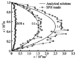
Fig.1 SPH simulation of Poiseuille flow with irregular particle distribution[38]

Fig.2 FPM simulation of Poiseuille flow with irregular particle distribution[38]
Liu and Liu[34]provided a comparative study of the kernel and particle consistency properties of the conventional SPH, CSPM and FPM, which are summarized in Table 1 and Table 2.

Table 1 Kernel consistency of SPH, CSPM, and FPM
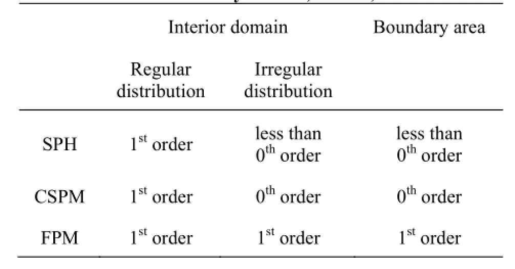
Table 2 Particle consistency of SPH, CSPM, and FPM

where xji=xj-xi, yji=yj-yi. If replacing ∇iWijon the RHS of Eq.(4) withWij, it is easy to show that for general cases with irregular particle distribution, variable smoothing length, and/or truncated boundary areas, the SPH particle approximation scheme for a gradient based on kernel gradient correction is of second order accuracy. It is noted that for kernel gradient correction, since only kernel gradient is corrected,there is no need to significantly change the structure of SPH computer programs and procedure of SPH simulations. It is therefore convenient to implement SPH equations of motion.
It is noted that both CSPM and FPM do not need to reconstruct smoothing function. Also in the conventional SPH method, a field function and its derivatives are approximated separately. Instead, in CSPM, the derivatives are approximated through solving a coupled matrix equation while the field function is approximated separately. In FPM, both the field function and its derivatives are coupled together and can be approximated simultaneously through solving a general matrix equation. As the solution of the general matrix equation can be tedious, Fang et al.[39]proposed a hybrid approach with the idea of using SPH approximation for the interior particles and FPM approximation for the exterior particles. Recently, Huang et al. developed an improved FPM, in which the kernel gradients need not to be calculated and this can make the selection of smoothing kernel function more flexible[40].
1.5Kernel gradient correction
Another popular improved SPH model is kernel gradient correction[41], from Eq.(4), it is known that the approximation accuracy of the derivatives is closely related to the accuracy of the gradient of the smoothing function (or kernel gradient). It is possible to use a corrective kernel gradient rather than the conventional kernel gradient in Eq.(4) to obtain better approximation accuracy. For example, in a two-dimensional space, based on Taylor series expansion on the SPH approximation of a function, it is possible to restore the accuracy for general cases with the following correction on the kernel gradient,

2. Modeling incompressible flows
2.1WCSPH
The governing equations for incompressible flow in Lagrangian frame can be written as:

where ρ, u, p, ν and F denote the density, the velocity, the pressure, the laminar viscosity and the external body force exerted on water, respectively.
In the standard SPH method for solving compressible flows, the particle motion is driven by the pressure gradient, while the particle pressure is calculated by the local particle density and internal energy through the equation of state. However, for incompressible flows, the actual equation of state of the fluid will lead to prohibitive time steps that are extremely small. How to effectively calculate the pressure term in the momentum equation is a major task for simulation of incompressible flows. Though it is possible to include the constraint of the constant density =0∇·u into SPH formulations, the resultant equations are usually too cumbersome.
In early SPH modeling of incompressible flow,an artificial compressibility technique is usually used to model the incompressible flow as a slightly compressible flow. The artificial compressibility considers that every theoretically incompressible fluid is actuallycompressible. Therefore, it is feasible to use a quasiincompressible equation of state (EOS) to model the incompressible flow. For this WCSPH approach, A frequently used artificial EOS is

where c is the sound speed which is a key factor that deserves careful consideration. If the actual sound speed is employed, the real fluid is approximated as an artificial fluid, which is ideally incompressible. Monaghan argued that the relative density variation δ is related to the fluid bulk velocity and sound speed in the following way[7]

where0ρ, ρΔ,bV and M are the initial density,absolute density variation, fluid bulk velocity and Mach number respectively.
It is clear that WCSPH is an explicit method and is similar to conventional SPH modeling of compressible flow. The difference is that in WCSPH, an artificial rather than true equation of state is used. As such,WCSPH solves the equations particle by particle without including the constraint of constant density.
2.2ISPH
It is noted that in WCSPH, an artificial equation of state should be used in modeling incompressible flow, and empirical values such as artificial sound need to be tuned. One possible problem is that the resultant pressure in conventional WCSPH is usually rough and oscillatory. Therefore, artificial viscosity and density corrections are usually used to obtain smooth pressure field[42,43]. As both the artificial compressibility and numerical artifacts involve empirical parameters, some researchers try to include the constraint of constant density into SPH method, somewhat similar to the moving particle semi-implicit method (MPS)[4,44]. This leads to projection-based incompressible smoothed particle hydrodynamics (ISPH) method[28,29]. Unlike WCSPH, the particle density in ISPH remains unchanged, ensuring the incompressibility of the modeling fluid. The pressure is implicitly obtained from solving the pressure Poisson's equation (PPE) rather than from an artificial equation of state as in WCSPH. The PPE is only related to the relative positions and relative velocities between particles without artificial parameters. Meanwhile, the solution of PPE in ISPH is based on the entire computational domain. Therefore compared with traditional WCSPH methods, the ISPH methods are usually said to be able to obtain much smoother pressure fields[45]. The pressure projection method is frequently applied in ISPH to ensure incompressibility. To reduce the occurrence of instability, a half-time step scheme is usually used[30,46]. In the first loop, the position and velocity of an SPH particle are firstly predicted.

where superscript * denotes the estimated value, n means the number of time step. After then, a correction step is applied based on the pressure force. Since the incompressibility ensures that the density does not change, the pressure of fluid particles and boundary particles are obtained by solving the following pressure Poisson equation

where the left-hand-side (LHS) can be expressed in SPH form as

The corrected velocity is then expressed as

The velocity and the position in half time step are obtained by:

The second loop in this numerical scheme advances another half time step to obtain the velocity and position at time step +1n.
2.3WCSPH vs ISPH
ISPH and WCSPH are two frequently used approaches in modeling incompressible flows within the frame of SPH. It is seen that ISPH is a semi-implicit method which needs to solve the pressure Poisson'sequation, and WCSPH is an explicit method which is based on the weakly compressible assumption of the incompressible fluid. Both methods have special advantages and disadvantages. There are several papers offering comparisons between ISPH and WCSPH. These papers compared the traditional WCSPH method and ISPH method and concluded that ISPH method has overall advantages over WCSPH method[47]. However, these works did not consider the recent improvements in the SPH method especially in correction of particle approximation, enhancements in the treatment of solid boundaries and free surfaces, and therefore the obtained conclusions are insufficient. Shadloo et al.[48]considered a robust WCSPH model and offered its comparison with ISPH method. But the presented numerical examples are not associated with changing and breakup of free surfaces, and violent fluid-solid interactions with liquid impact, sloshing and splashing. These are usually the most important features for violent free surface flows with moving objects.
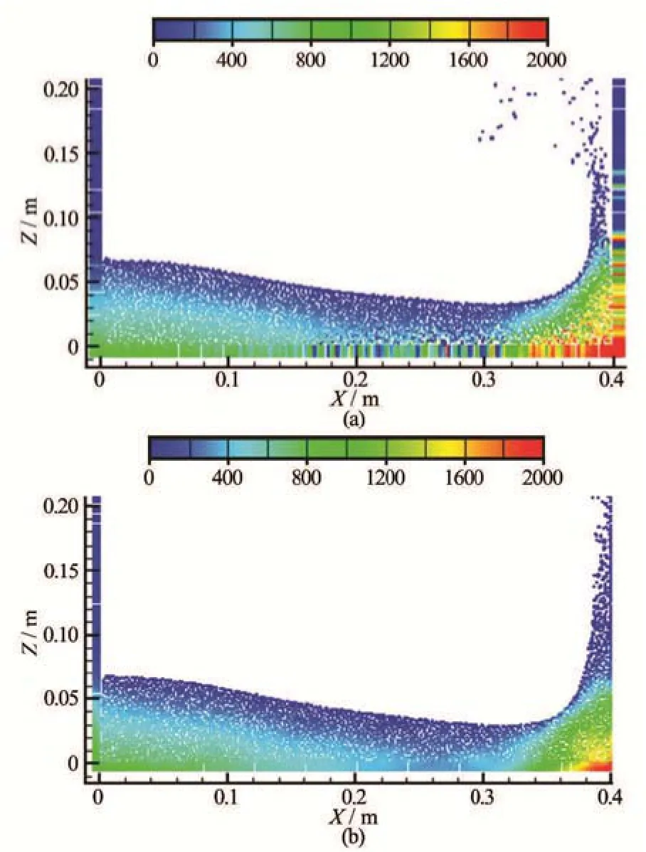
Fig.3 (Color online) ISPH (a) and SPH (b) modeling of a dam breaking problem. ISPH is more sensitive to numerical oscillations and easier to induce numerical instability[30]
As ISPH and WCSPH are very popular, while reported results are usually inconsistent, Chen et al.[30]conducted a comprehensive study of the ISPH method and an improved weakly compressible SPH method in free surface flows (see Fig.3). Both methods solve the Navier-Stokes equations in Lagrangian form and no artificial viscosity is used. The ISPH algorithm presented in their work is based on the classical SPH projection method with some common treatments on solid boundaries and free surfaces. The WCSPH model includes some advanced corrective algorithms in density approximation and solid boundary treatment. They found that although ISPH can use much bigger time steps, it needs to solve the time-consuming sparse matrix equation. Therefore ISPH is not superior to IWCSPH in computational cost. For problems with a large number of particles, WCSPH can even be more efficient than ISPH. For problems with violent water impact and fluid-structure interactions, WCSPH is more accurate and more stable while ISPH is more sensitive to numerical oscillations and is easier to cause instability. Using improved approximation schemes as discussed in Section 2 in WCSPH can lead to better performance. This may be the reason that there are many more works on WCSPH rather than on ISPH when modeling incompressible viscous flows. It is also noted that the original MPS method which solves the pressure Possion's equation in a way similar to ISPH gradually uses the concept of artificial compressibility to model incompressible flows[49].
3. Treatment of solid boundaries
Particle methods such as molecular dynamics(MD), dissipative particle dynamics (DPD), and SPH are very different from the grid-based numerical methods in treating solid boundary, and care must be taken in this regards. For finite element methods,proper boundary conditions can be well defined and properly imposed without affecting the stability of the disrete model. In the finite difference method, because the domain is relatively regular, proper ways to handling the boundary conditions have already been developed. In either FEM or FDM, the implementations of boundary conditions (either Neumann boundary conditions or Dirichlet boundary conditions, or mixed boundary conditions) are generally straightforward[50,51]. In contrast, in MD, DPD and SPH, the implementation of the boundary conditions is not as straightforward as in the grid-based numerical models. This has been regarded historically as one weak point of the particle methods[52-56]. For molecular dynamics and dissipative particle dynamics, it is common to fill the solid obstacle areas with frozen particles. These fixed particles can prevent the mobile particles from penetrating the solid walls, and interact with the mobile particles with proper interaction models. Different complex solid matrix and solid-fluid interface physics can thus be modeled by appropriately deploying fixed particles plus a suitable interaction model with mobile particles. Preventing fluid particles from penetrating solid walls by exerting a repulsive force simulates the boundary condition with zero normal velocity. Different models of reflection or mirror of fluid particles orinteraction models of solid particles with fluid particles can also be applied to exert slip or non-slip boundary condition. In principal, the boundary treatment techniques in MD and DPD can also be used for SPH. However, SPH is a continuum scale particle method,and the field variables on boundaries such as pressure need to be directly calculated. Therefore solid boundary treatment in SPH is more difficult and numerical techniques for implementing solid wall boundary conditions are also more diversified.
To well implement the solid boundary conditions and improve the numerical accuracy, many researchers have proposed different solid boundary treatment(SBT) algorithms for the SPH method. Except for approaches with coupled grid-based methods, which can take the advantages in dealing with solid boundaries, most SBT algorithms use virtual particles (or ghost or image particles in different references) to represent the solid boundary (and even the solid obstacle areas). Depending on the deployment of the virtual particles and numerical approximation schemes to obtain field variables of the corresponding virtual particles, these SBT algorithms can be classified into three major classes, repulsive force SBT, dynamic SBT and conventional SBT algorithms with ghost particles.
3.1Repulsive force SBT algorithm
The repulsive force SBT algorithm was first used by Monaghan[57]who used a line of virtual particles(as repulsive particles) located right on the solid boundary to produce a highly repulsive force on the approaching fluid particles near the boundary, and thus to prevent these fluid particles from unphysical penetration through solid boundaries, as shown in Fig.4.

Fig.4 Illustration of the repulsive force SBT algorithm
The early repulsive force is very much similar to the Lennard-Jones (LJ) formmolecular force in classic molecular dynamics. The LJ form repulsive force is very strong and usually may produce large numerical oscillation in the solid boundary area[35,58]. Later other forms of repulsive force are used and these force models are usually softer than the LJ force model. For example, an improved repulsive force model is given by Rogers and Dalrymple[59]in modeling tsunami waves and run-up. Except for distance between particles, normal and tangential directions are necessary to be determined before calculating the repulsive force.
3.2Dynamic SBT algorithm
The idea of dynamic boundary treatment was mentioned in Liu and Liu's SPH monograph[20], and was also implemented by Dalrymple and his co-workers in modeling free surface flows[10,60]. In dynamic SBT algorithms, virtual particles are placed and fixed in the boundary area, and the thickness of the virtual boundary particles is related to the kernel function as well as initial particle spacing (see Fig.5). Virtual particles are used to approximate the field variables of fluid particles, and thus to improve the SPH numerical accuracy near boundary areas through removing the boundary deficiency problem. On the other hand, field variable of the virtual particles can be obtained DYNAMICALLY from SPH approximation on governing equations such as the continuity equation, momentum equation and the equation of state. Since field variables of the virtual particles are dynamically evolved according to the governing equations, the involved solid boundary treatment is usually referred to as dynamic SBT.

Fig.5 Illustration of the dynamic SBT algorithm
The dynamic SBT algorithm improves computational accuracy by removing the particle deficiency problem for fluid particles, and it is also suitable for complex solid boundaries. But in many cases, fluid particles may unphysically penetrate the solid walls.It is noted that when approximating field variables of virtual particles, numerical problems with boundary deficiency still exist. As for a concerned virtual particle, there are not sufficient particles in its support domain to take part in the weighted summation process. Therefore the dynamic SBT algorithm can also lead to inaccurate results with pressure oscillations. Gong et al.[61]proposed an improvement in smoothing the pressure field in their dynamic SBT algorithm, and it is reported to have better performance, especially in removing pressure oscillations.

Fig.6 Illustration of the ghost particle SBT algorithm
3.3Ghost particle SBT algorithm
SBT algorithms with ghost particles have been frequently used in SPH.In this method, ghost particles are generated to represent the solid boundary areas by mirroring or reflecting fluid particles along solid boundaries (Fig.6). A line of boundary particles may also be used to exert repulsive forces. Ghost particles can be generated only once at the first time step, andfixed in the computational domain for later approximations. They can also be generated at each time step and adapt with changing neighbor fluid particles. Ghost particles can take part in the SPH approximation process of the fluid particles to improve boundary accuracy, while different ways to obtain the field variables can lead to different implementations.
Libersky and his co-workers[62]introduced ghost particles to reflect a symmetrical surface boundary condition with opposite velocity on the reflecting image particles. Colagrossi and Landrini[63]used an approach to mimic the solid boundary by ghost particle with density, pressure and velocity from neighbor fluid particles. Morris et al.[64]proposed an approach to obtain velocity of virtual boundary particles for implementing non-slip boundary conditions. Particles are created on a regular lattice, and contribute to the computation of the density and pressure gradients of fluid particles. The velocities of the boundary particles are obtained through the ratios of the distances from real particles and boundary particles to the boundary. Marrone and Colagrossi and Colagrossi[65]proposed an improved SBT algorithm with fixed ghost particle and used it to simulated dam break problems. The solid boundary is represented by several layers of fixed ghost particles. To obtain variables (such as density,pressure and velocity) of a fixed ghost particle, it is necessary to introduce an image interpolation point by reflecting a concerned ghost particle to the flow region.
It is noted that ghost particle SBT algorithmsare usually applicable only to simple or straightforward boundaries in order to generate ghost particles. The SBT algorithmby Marrone and Colagrossi[65]is actually a combination of the dynamic SBT algorithm and the ghost particle SBT algorithms. Thus it can lead to comparatively better results.

Fig.7 Illustration of the coupled dynamic SBT algorithm
3.4Coupled dynamic SBT algorithm
Recently Liu et al.[31]proposed a coupled dynamic SBTalgorithm, in which two types of virtual particles, repulsive particles and ghost particles (as shown in Fig.7), are used to represent the solid boundary. The repulsive particles produce a suitable repulsive force to the approaching fluid particles near the boundary,and they are located right on the solid boundary. Ghost particles are located outside the solid boundary area. Different from conventional ghost particle SBT algorithms, in which ghost particles are generated by mirroring or reflecting fluid particles onto solid boundary areas, and need to adapt with the fluid particles at each time step, this new SBT algorithm can generates ghost particles in a regular or irregular distribution at the first time step, while ghost particle positions do not need to change during following steps.
The coupled dynamic SBT algorithm consists of a soft repulsive force for repulsive particles, and a high order scheme to approximate the information of the virtual particles. The new repulsive force is a distance-dependent repulsive force with finite magnitude on fluid particles approaching solid boundaries. It is an improvement on Koumoutsakos's work[66], which needs to calculate the tangential and normal directions of solid boundaries, and is not easy to implement for complex geometries. The improved repulsive force is a finite distance-dependent repulsive force on fluid particles approaching solid boundaries. To restore the consistency of SPH particle approximation, Shepard filter method or moving least square (MLS) method can be used in the coupled dynamic SBT algorithm for approximating both the fluid and virtual particles.
Figure 8 shows the pressure (left) and particle(right, zoom-in plots) distributions obtained using the repulsive force, dynamic and coupled dynamic SBT algorithms[31]. It is obvious that repulsive force and dynamic SBT algorithms lead to rough pressure field with numerical oscillations especially in the bottomright corner area. Also for both SBT algorithms, a clear particle separation can be observed near the topright solid wall. It is therefore difficult to obtain accurate pressure loads on the solid boundary due to pressure oscillation and particle separation. In contrast,the pressure distribution obtained from the coupled dynamic SBT algorithm leads to more ordered particle distribution and much smoother pressure field with clear pressure layers. Large impact pressure in the corner area can be effectively predicted with obvious pressure layers.

Fig.8 (Color online) Particle and pressure distributions obtained using three SBT algorithms[31]
4. Particle adapting or shifting
SPH usually suffers from low accuracy due to the highly disordered particle distribution when modeling incompressible flow with violently evolving free surfaces. One possible way to improve computational accuracy is to use high order approximation schemes as discussed in Section 2. However, in these high order SPH approximation schemes, a corrective matrix is usually involved at each particle for every time step and this is computationally expansive. Moreover, for extremely disorder particle distribution, the corrective matrix may be ill-conditioned without inverse and this can cause numerical instability. As the conventional SPH method is simple, stable, and has second order accuracy for regularly distributed interior particles,some researchers proposed algorithms to adapt or shift particle positions so as to make the irregularly distributed particle (roughly) regular or even and therefore to improve the computational accuracy of the conventional SPH method. Typical of them include the XSPH and particle shifting algorithm (PSA).
4.1XSPH
The XSPH technique was proposed by Monaghan[24,25]. In XSPH, SPH particle moves in the following way

where ε is a constant in the range of 01.0ε≤≤. It is clear that the XSPH technique includes the contribution from neighboring particles, and thus makes the particle move in a velocity closer to the average velocity of the neighboring particles. The XSPH technique,when applied to incompressible flows, can keep the particles more orderly, when applied to compressible flows, can effectively reduce unphysical penetration between approaching particles. In most circumstances ε=0.3 seems to be a good choice in simulating incompressible flows. The XSPH technique will also be applied in the simulation of explosions, in which a larger value (0.5)ε≥ can be used[20,67].
4.2Particle shifting algorithm
The particle shifting algorithm was first proposed by Xu, Lind and their co-workers[26,27]to resolve the numerical instability in a projection based ISPH method. The PAS algorithm is based on Fick's law of diffusion and shifts particles to prevent highly anisotropic distributions and the onset of numerical instability. As PSA is effective in obtaining noise-free pressure fields, it is popular in recent SPH modeling of free surface flows.
In general, PSA consists of two steps. In the first step, the shifting vector (δri) of particle i can by obtained from following equation

where C is a constant in the range of 0.01-0.1, ζ andiR are the shifting magnitude and direction of particle i, which can be calculated as follows:

wheremaxV is the maximal particle velocity, tΔ is the time step, ijr is the spacing between particle i and j, nijis the unit displacement vector,is the average particle spacing in the neighborhood of particle

In the second step, after the particles are shifted to the new positions according to Eq.(28), field variables must be corrected accordingly as whereiψ'andiψ denote a field variable (i.e., density,pressure, velocity, position) after and before particle shifting.
5. Concluding remarks
As a meshfree, Lagrangian particle method, SPH is popular in modeling viscous incompressible flows with possible interacting structures. This paper provides a review on the recent developments of SPH in modeling viscous incompressible flows in four major aspects including SPH particle approximation schemes,pressure field solution approaches, solid boundary treatment algorithms and particle adapting algorithms.
The SPH particle approximation scheme determines the discretization accuracy of a field function and its derivatives. A number of improved approximation schemes are available now, which are superior to the conventional SPH approximation scheme in accuracy. Approaches which improve the computational accuracy without changing the conventional smoothing function are usually more preferable in simulating viscous incompressible flows. These approaches in general originates from Taylor series analysis of the SPH kernel approximation of a field function and its derivatives, while different treatments lead to different modified versions such as CSPM and FPM. FPM canbe regarded as the improved version of both SPH and CSPM and if only the gradients of a field function are concerned, FPM can be transformed into KGC, which is also straightforward and popular in modeling viscous incompressible flows.
Such improved SPH approximation schemes usually involve a corrective matrix, which can be illconditioned for extremely disordered particles. Therefore some algorithms such as XSPH and PSA to adapt or shift particle positions so as to make the irregularly distributed particle (roughly) regular or even are attractive as these approaches are simple to implement and can improve computational accuracy in many circumstances. XSPH is more empirical, while PSA has comparatively solid theoretical basis and therefore it is more reliable. It is noted that both XSPH and PSA involve some kind of average on field variables when adapting particle positions. This may lead to “smoothed” rather than “physical” results for problems with discontinuities (e.g., cracks, shocks and etc.) in which the uneven particle distribution is physical.
For the solution of pressure field, two distinct approaches, WCSPH and ISPH, are comparatively discussed. Theoretically ISPH can obtain smoother pressure field as the pressure is strictly obtained from solving the pressure Poisson's equation rather than using the assumption of weak compressibility as in WCSPH. However, as the compressibility is a fluid physics and if the artificial sound speed and equation are well selected, WCSPH can be more attractive than ISPH since WCSPH is simpler and more stable with comparable or even better accuracy and less computational efforts.
SPH simulations have also suffered from not being able to directly implement the solid boundary conditions. This influences the SPH approximation accuracy and hinders its further development and application to engineering and scientific problems. This paper reviews four typical solid boundary treatment algorithms, i.e., the repulsive force SBT algorithm, the dynamics SBT algorithm, the ghost particle SBT algorithm and the coupled dynamics SBT algorithm. As the coupled dynamics SBT algorithm includes a kernel-style soft repulsive force between approaching fluid and solid particles, there will not be large numerical oscillation near the boundary while unphysical particle penetration can be well prevented. Also the coupled dynamics SBT algorithm using improved particle approximation schemes such as FPM or KGC for estimating field functions of virtual solid particles, it is more accurate in boundary area.
6. Future works
Except for the above-mention aspects, several other issues need to be taken into account when modeling viscous incompressible flows, including turbulence modeling, coupling approaches and computational efficiency.
Turbulence modeling: Turbulence modeling is an important aspect in the simulation of viscous incompressible flows, especially for breaking waves and for problems with strong FSIs, in order to get very refined information about the velocities, turbulence, and transport properties. Direct numerical simulation (DNS)[68]has very high accuracy, however this method needs so many particles and currently it is not practical to simulate complex flow fields with large computational domain for SPH. During the last decades, different turbulence models have been incorporated into SPH method, while most of them are based on large eddy simulation (LES) or Reynolds averaged Navier-Stokes(RANS). For example, Shao and Ji presented a 2-D LES modeling approach in SPH to investigate the properties of the plunging waves and they demonstrated that both the turbulence model and the spatial resolution play an important role in the model predictions[69]. Liu and his co-workers used the RANS approach to study the turbulence and vortex during liquid sloshing[41]. As the RANS approach may overestimate the turbulence level[70], it must be cautious when using this approach for some special applications. LES lies between the extremes of DNS and RANS modelling and attempts to capture the large-scale motion with most of the energies and momentums without too much effort, and therefore it can be a good choice for turbulence modeling with SPH.
Coupling approaches: Though SPH has special advantages in modeling viscous incompressible flows,it is associated with some drawbacks that need to be improved. The conventional SPH is flexible and stable with adaptive nature, while it is of low accuracy. Most of the improved SPH models are associated with good accuracy while they usually meet instability especially when particles are highly irregular. Also treatment of solid boundary in particle-based methods in general is not as accurate, easy and straightforward as grid-based methods. Therefore, during the last decades, many different approaches have been proposed to couple SPH with grid-based methods. The very early examples are to couple SPH with FEM for modeling impact problems by Johnson and his co-workers[71,72]. Some recent examples are the effort in coupling SPH with FEM for fluid-structure interactions with viscous incompressible flows[73-75]or with finite volume method for free surface flows[76]. Another trend is to couple SPH with other particle-based methods for different purposes. For example, SPH is coupled with discrete element method (DEM)[77]for simulating environmental flows in which SPH is used for modeling the fluid flows and DEM is used to model granular flows[78,79]. SPH is also coupled with peridynamics (PD)[80]for simulating soil fragmentation by blast loads of buried explosive[81].
Computational efficiency: Modeling of viscous incompressible flows with SPH has been associated with the comparatively low computational efficiency due to the heavy cost in particle-particle interaction calculations, which is a common feature for particlebased methods such as molecular dynamics and dissipative particle dynamics. This heavy computational cost, on one hand, can be slightly alleviated with efficient particle searching algorithms such as link-list and tree search algorithms or different improved versions[20,82,83], on the other hand, can be greatly reduced by using state-of-the-art high performance computing(HPC) techniques. One special advantage is that as a Lagrangian particle method, SPH is well suited for HPC and its computational performance can be can be greatly enhanced using parallel computing techniques such as message passing interface (MPI) and graphic processing unit (GPU)[84,85]. Therefore using HPC techniques in SPH for modeling viscous incompressible flows is necessary, especially for engineering problems.
References
[1]HIRT C., NICHOLS B. Volume of fluid (VOF) method for the dynamics of free boundaries[J]. Journal of Computational Physics, 1981, 39(1): 201-225.
[2]SETHIAN J. Level set methods and fast marching methods[J]. Journal of Computing and Information Technology, 2003, 11(1): 1-2.
[3]HU C., KASHIWAGI M. A CIP-based method for numerical simulations of violent free-surface flows[J]. Journal of Marine Science and Technology, 2004, 9(4): 143-157.[4]KOSHIZUKA S., OKA Y. Moving-particle semi-implicit method for fragmentation of incompressible fluid[J]. Nuclear Science and Engineering, 1996, 123(3): 421-434.
[5]GINGOLD R. A., MONAGHAN J. J. Smoothed particle hydrodynamics-Theory and application to non-spherical stars[J]. Monthly Notices of The Royal Astronomical Society, 1977, 181(3): 375-389.
[6]LUCY L. B. A numerical approach to the testing of the fission hypothesis[J]. Astronomical Journal, 1977, 82(2): 1013-1024.
[7]MONAGHAN J. J. Simulating free surface flows with SPH[J]. Journal of Computational Physics, 1994, 110(2): 399-406.
[8]LO Y. M. E., SHAO S. Simulation of near-shore solitary wave mechanics by an incompressible SPH method[J]. Applied Ocean Research, 2002, 24(5): 275-286.
[9]SAMPATH R., MONTANARI N. and AKINCI N. et al. Large-scale solitary wave simulation with implicit incompressible SPH[J]. Journal of Ocean Engineering and Marine Energy, 2016, 2(3): 1-17.
[10] GOMEZ-GESTEIRA M., DALRYMPLE R. A. Using a three-dimensional smoothed particle hydrodynamics method for wave impact on a tall structure[J]. Journal of Waterway Port Coastal And Ocean Engineering, 2004,130(1): 63-69.
[11] AMINI Y., EMDAD H. and FARID M. A new model to solve fluid-hypo-elastic solid interaction using the smoothed particle hydrodynamics (SPH) method[J]. European Journal of Mechanics-B/Fluids, 2011, 30(2): 184-194.
[12] CUMMINS S., SILVESTER T. and CLEARY P. W. Three-dimensional wave impact on a rigid structure using smoothed particle hydrodynamics[J]. International Journal for Numerical Methods in Fluids, 2012, 68(12): 1471-1496.
[13] MARUZEWSKI P., TOUZD. L. and OGER G. et al. SPH high-performance computing simulations of rigid solids impacting the free-surface of water[J]. Journal of Hydraulic Research, 2010, 48(Supp1.): 126-134.
[14] GMEZ-GESTEIRA M., CERQUEIRO D. and CRESPO C. et al. Green water overtopping analyzed with a SPH model[J]. Ocean Engineering, 2005, 32(2): 223-238.
[15] MARRONE S., COLAGROSSI A. and ANTUONO M. et al. An accurate SPH modeling of viscous flows around bodies at low and moderate Reynolds numbers[J]. Journal of Computational Physics, 2013, 245(1): 456-475.
[16] KHORASANIZADE S., SOUSA J. M. A detailed study of lid-driven cavity flow at moderate Reynolds numbers using Incompressible SPH[J]. International Journal for Numerical Methods in Fluids, 2014, 76(10): 653-668.
[17] GOMEZ-GESTEIRA M., ROGERS B. D. and DALRYMPLE R. A. et al. State-of-the-art of classical SPH for freesurface flows[J]. Journal of Hydraulic Research, 2010,48(Supp1): 6-27.
[18] LIU W. K., CHEN Y. and JUN S. et al. Overview and applications of the reproducing kernel particle methods[J]. Archives of Computational Methods in Engineering,1996, 3(1): 3-80.
[19] LIU W. K., JUN S. and LI S. et al. Reproducing kernel particle methods for structural dynamics[J]. International Journal for Numerical Methods in Engineering, 1995,38(10): 1655-1679.
[20] LIU G. R., LIU M. B. Smoothed particle hydrodynamics: A meshfree particle method[M]. Singapore: World Scientific, 2003.
[21] LIU M. B., LIU G. R. and LAM K. Y. Constructing smoothing functions in smoothed particle hydrodynamics with applications[J]. Journal of Computational and Applied Mathematics, 2003, 155(2): 263-284.
[22] CHEN J. K., BERAUN J. E. A generalized smoothed particle hydrodynamics method for nonlinear dynamic problems[J]. Computer Methods in Applied Mechanics and Engineering, 2000, 190(1): 225-239.
[23] BONET J., KULASEGARAM S. Correction and stabilization of smooth particle hydrodynamics methods with applications in metal forming simulations[J]. International Journal for Numerical Methods in Engineering, 2000,47(6): 1189-1214.
[24] MONAGHAN J. J. On the problem of penetration in particle methods[J]. Journal of Computational Physics, 1989,82(1): 1-15.
[25] MONAGHAN J. J. Smooth particle hydrodynamics[J]. Annual Review of Astronomy and Astrophsics, 1992,30: 543-574.
[26] LIND S., XU R. and STANSBY P. et al. Incompressible smoothed particle hydrodynamics for free-surface flows: A generalised diffusion-based algorithm for stability and validations for impulsive flows and propagating waves[J]. Journal of Computational Physics, 2012, 231(4): 1499-1523.
[27] XU R., STANSBY P. and LAURENCE D. Accuracy and stability in incompressible SPH (ISPH) based on the projection method and a new approach[J]. Journal of Computational Physics, 2009, 228(18): 6703-6725.
[28] CUMMINS S. J., RUDMAN M. An SPH projection me-thod[J]. Journal of Computational Physics, 1999, 152(2): 584-607.
[29] RAFIEE A., THIAGARAJAN K. P. An SPH projection method for simulating fluid-hypoelastic structure interaction[J]. Computer Methods in Applied Mechanics and Engineering, 2009, 198(33): 2785-2795.
[30] CHEN Z., ZONG Z. and LIU M. B. et al. A comparative study of truly incompressible and weakly compressible SPH methods for free surface incompressible flows[J]. International Journal for Numerical Methods in Fluids,2013, 73(9): 813-829.
[31] LIU Mou-bin, SHAO Jia-ru. and CHANG Jian-zhong. On the treatment of solid boundary in smoothed particle hydro-dynamics[J]. Science China Technological Sciences, 2012, 55(1): 244-254.
[32] MONAGHAN J. J. Smoothed particle hydrodynamics[J]. Reports on Progress in Physics, 2005, 68(8): 1703-1759.[33] LIU M. B., XIE W. P. and LIU G. R. Modeling incompressible flows using a finite particle method[J]. Applied Mathematical Modelling, 2005, 29(12): 1252-1270.
[34] LIU M. B., LIU G. R. Restoring particle consistency in smoothed particle hydrodynamics[J]. Applied Numerical Mathematics, 2006, 56(1): 19-36.
[35] LIU M. B., LIU G. R. Smoothed particle hydrodynamics(SPH): An overview and recent developments[J]. Archives of Computational Methods in Engineering, 2010,17(1): 25-76.
[36] DILTS G. A. Moving-least-squares-particle hydrodynamics-I. Consistency and stability[J]. International Journal for Numerical Methods in Engineering, 1999, 44(8): 1115-1155.
[37] RANDLES P. W., LIBERSKY L. D. Smoothed particle hydrodynamics: Some recent improvements and applications[J]. Computer Methods in Applied Mechanics and Engineering, 1996, 139(1-4): 375-408.
[38] LIU Mou-bin, CHANG Jian-zhong. Particle distribution and numerical stability in smoothed particle hydrodynamics[J]. Acta Physica Sinica, 2010, 59(6): 3654-3662(in Chinese).
[39] FANG J., PARRIAUX A. and RENTSCHLER M. et al. Improved SPH methods for simulating free surface flows of viscous fluids[J]. Applied Numerical Mathematics,2009, 59(2): 251-271.
[40] HUANG C., LEI J. M. and LIU M. B. et al. A kernel gradient free (KGF) SPH method[J]. International Journal for Numerical Methods in Fluids, 2015, 78(11): 691 -707.
[41] SHAO J. R., LI H. Q. and LIU G. R. et al. An improved SPH method for modeling liquid sloshing dynamics[J]. Computers and Structures, 2012, 100-101(6): 18-26.
[42] COLAGROSSI A., LANDRINI M. Numerical simulation of interfacial flows by smoothed particle hydrodynamics[J]. Journal of Computational Physics, 2003, 191(2): 448-475.
[43] LIU M. B., SHAO J. R. and LI H. Q. An SPH model for free surface flows with moving rigid objects[J]. International Journal for Numerical Methods in Fluids, 2014,74(9): 684-697.
[44] KOSHIZUKA S., NOBE A. and OKA Y. Numerical analysis of breaking waves using the moving particle semiimplicit method[J]. International Journal For Numerical Methods In Fluids, 1998, 26(7): 751-769.
[45] LIU X., XU H. and SHAO S. et al. An improved incompressible SPH model for simulation of wave-structure interaction[J]. Computers and Fluids, 2013, 71: 113-123.
[46] BCKMANN A., SHIPLIOVA O. and SKEIE G. Incompressible SPH for free surface flows[J]. Computers and Fluids, 2012, 67: 138-151.
[47] LEE E.-S., MOULINEC C. and XU R. et al. Comparisons of weakly compressible and truly incompressible algorithms for the SPH mesh free particle method[J]. Journal of Computational Physics, 2008, 227(18): 8417-8436.
[48] SHADLOO M. S., ZAINALI A. and YILDIZ M. et al. A robust weakly compressible SPH method and its comparison with an incompressible SPH[J]. International Journal for Numerical Methods in Engineering, 2012, 89(8): 939-956.
[49] SHAKIBAEINIA A., JIN Y.-C. A weakly compressible MPS method for modeling of open-boundary free-surface flow[J]. International Journal for Numerical Methods in Fluids, 2010, 63(10): 1208-1232
[50] ZIENKIEWICZ O. C., TAYLOR R. L. The finite element method[M]. Oxford, UK: Butterworth-Heinemann,2000.
[51] HIRSCH C. Numerical computation of internal and external flows: Fundamentals of numerical discretization[M]. New York, USA: John Wiley and Sons, 1988.
[52] AGERTZ O., MOORE B. and STADEL J. et al. Fundamental differences between SPH and grid methods[J]. Monthly Notices of The Royal Astronomical Society, 2007,380(3): 963-978.
[53] SCHUSSLER M., SCHMITT D. Comments on smoothed particle hydrodynamics[J]. Astronomy and Astrophysics,1981, 97: 373-379.
[54] HERNQUIST L. Some cautionary remarks about smoothed particle hydrodynamics[J]. Astrophysical Journal,1993, 404(2): 717-722.
[55] NGUYEN V. P., RABCZUK T. and BORDAS S. et al. Meshless methods: A review and computer implementation aspects[J]. Mathematics and Computers in Simulation, 2008, 79(3): 763-813.
[56] REVENGA M., ZUNIGA I. and ESPANOL P. Boundary models in DPD[J]. International Journal of Modern Physics C, 1998, 9(8): 1319-1328.
[57] MONAGHAN J. J. Simulating free-surface flows with SPH[J]. Journal of Computational Physics, 1994, 110(2): 399-406.
[58] LIU M. B., LIU G. R. Particle methods for multiscale and multiphysics[M]. Singapore: World Scientific, 2015.
[59] ROGERS B., DALRYMPLE R. SPH modeling of tsunami waves[J]. Advanced Numerical Models for Simulating Tsunami Waves and Runup, 2007, 10: 75-100.
[60] LIU M. B., LIU G. R. Smoothed particle hydrodynamics(SPH): An overview and recent developments[J]. Archives of Computational Methods in Engineering, 2010,17(1): 25-76.
[61] GONG Kai, LIU Hua and WANG Ben-long. Water entry of a wedge based on SPH model with an improved boundary treatment[J]. Journal of Hydrodynamics, 2009,27(6): 750-757.
[62] LIBERSKY L. D., PETSCHEK A. G. and CARNEY T. C. et al. High-strain lagrangian hydrodynamics-A threedimensional SPH code for dynamic material responses[J]. Journal of Computational Physics, 1993, 109(1): 67-75.
[63] COLAGROSSI A., LANDRINI M. Numerical simulation of interfacial flows by smoothed particle hydrodynamics[J]. Journal of computational physics, 2003, 191(2): 448-475.
[64] MORRIS J., FOX P. and ZHU Y. Modeling low Reynolds number incompressible flows using SPH[J]. Journal of Computational Physics, 1997, 136(1): 214-226.
[65] MARRONE S., COLAGROSSI A. Delta SPH model for simulating violent impact flows[J]. Computer Methods in Applied Mechanics and Engineering, 2011, 200(13-16): 1526-1542.
[66] KOUMOUTSAKOS P. Multiscale flow simulations using particles[J], Annual Review of Fluid Mechanics, 2005,37(1): 457-487.
[67] LIU M. B., LIU G. R. and ZONG Z. et al. Computer simulation of high explosive explosion using smoothed particle hydrodynamics methodology[J]. Computers and Fluids,2003, 32(3): 305-322.
[68] MOIN P., MAHESH K. Direct numerical simulation: A tool in turbulence research[J]. Annual Review of Fluid Mechanics, 1998, 30(1): 539-578.
[69] SHAO S. Incompressible SPH simulation of wave breaking and overtopping with turbulence modelling[J]. International Journal for Numerical Methods in Fluids,2006, 50(5): 597-621.
[70] LIN P., LIU P. L. F. A numerical study of breaking waves in the surf zone[J], Journal of Fluid Mechanics, 1998,359(1): 239-264.
[71] JOHNSON G. R. Linking of Lagrangian particle methods to standard finite element methods for high velocity impact computations[J]. Nuclear Engineering and Design,1994, 150(2-3): 265-274.
[72] JOHNSON G. R., STRYK R. A. and BEISSEL S. R. SPH for high velocity impact computations[J]. Computer Methods in Applied Mechanics and Engineering, 1996,139(1): 347-373.
[73] HU D., LONG T. and XIAO Y. et al. Fluid-structure interaction analysis by coupled FE-SPH model based on a novel searching algorithm[J]. Computer Methods in Applied Mechanics and Engineering, 2014, 276: 266-286.
[74] ZHANG A. M., MING F. R. and WANG S. P. Coupled SPHS-BEM method for transient fluid-structure interaction and applications in underwater impacts[J]. Applied Ocean Research, 2013, 43(10): 223-233.
[75] LEE C. J. K., NOGUCHI H. and KOSHIZUKA S. Fluid shell structure interaction analysis by coupled particle and finite element method[J]. Computers and Structures,2007, 85(11-14): 688-697.
[76] MARRONE S., MASCIO A. D. and TOUZE D. L. Coupling of smoothed particle hydrodynamics with finite volume method for free surface flows[J]. Journal of Computational Physics, 2016, 310(3): 161-180.
[77] CUNDALL P. A., STRACK O. D. L. A discrete numerical model for granular assemblies[J]. Geotechnique, 1979,29(1): 47-65.
[78] ZEGHAL M., SHAMY U. E. Coupled continuum-discrete model for saturated granular soils[J]. Journal of Engineering Mechanics, 2005, 131(4): 413-426.
[79] CLEARY P. W., PRAKASH M. Discrete-element modelling and smoothed particle hydrodynamics: Potential in the environmental sciences[J]. Philosophical Transactions: Mathematical, Physical and Engineering Sciences,2004, 362(1822): 2003-2030.
[80] SILLING S. A., ASKARI E. A meshfree method based on the peridynamic model of solid mechanics[J]. Computers and Structures, 2005, 83(17): 1526-1535.
[81] FAN H., BERGEL G. L. and LI S. A hybrid peridynamics-SPH simulation of soil fragmentation by blast loads of buried explosive[J]. International Journal of Impact Engineering, 2015, 86: 14-27.
[82] CAI Y., ZHU H. A local search algorithm for natural neighbours in the natural element method[J]. International Journal of Solids and Structures, 2005, 42(23): 6059-6070.
[83] BATRA R. C., ZHANG G. M. Search algorithm, and simulation of elastodynamic crack propagation by modified smoothed particle hydrodynamics (MSPH) method[J]. Computational Mechanics, 2007, 40(3): 531-546.
[84] VALDEZ-BALDERAS D., DOM NGUEZ J. M. and ROGERS B. D. et al. Towards accelerating smoothed particle hydrodynamics simulations for free-surface flows on multi-GPU clusters[J]. Journal of Parallel And Distributed Computing, 2013, 73(11): 1483-1493.
[85] DOM NGUEZ J. M. and CRESPO A. J. et al. Optimization strategies for CPU and GPU implementations of a smoothed particle hydrodynamics method[J]. Computer Physics Communications, 2013, 184((3): 617-627.
E-mail: mbliu@pku.edu.cn
(September 20, 2016, Revised September 24, 2016)
* Project supported by the National Natural Science Foundation of China (Grant Nos. 11172306, U1530110), the Institute of Systems Engineering, China Academy of Engineering Physics (Grant No. 2013KJZ01).
Biography: Mou-bin LIU (1970-), Male, Ph. D., Professor

- 水动力学研究与进展 B辑的其它文章
- Sharp interface direct forcing immersed boundary methods:A summary of some algorithms and applications*
- Flow characteristics of the wind-driven current with submerged and emergent flexible vegetations in shallow lakes*
- Reverse motion characteristics of water-vapor mixture in supercavitating flow around a hydrofoil*
- Study of fluid resonance between two side-by-side floating barges*
- Modelling of a non-buoyant vertical jet in waves and currents*
- Investigation on lane-formation in pedestrian flow with a new cellular automaton model*