构建AP-HTPB固体推进剂松弛模量主曲线的不同方法

Walid M Adel, 梁国柱

(北京航空航天大学宇航学院, 北京100083 )

1 Introduction

The solid propellant exhibits very complicated viscoelastic behavior and its mechanical properties (the relationship between tension and stress) and failure mechanisms are really sensible at the time of application loads, and temperature change. Relaxation modulus is one of the most important mechanical properties of viscoelastic materials which can be used to simulate the viscoelastic material behavior[1]. The master curve of the relaxation modulus is defined as the relationship between the relaxation modulus and the reduced loading time and it is constructed based on a selected reference temperature of interest to which all data must be shifted using shift factors. The shift factor is defined as a unique parameter which takes into account both the temperature and strain rate effects of the temperature of interest relative to the reference temperature[2]. Depending on a master curve, the mechanical properties and the behavior of composite solid propellant can be predicted at different times and temperatures based on a limited set of experimental data. This anticipation is often performed through basic time-temperature superposition (TTS) principle.

The related publications in the extant literature, primarily concentrate on the application of TTS principle of solid propellant under different loading conditions. Chyuan analyzed numerically the structural integrity of HTPB solid propellant grains subjected to temperature loading[3], ignition pressurization loading[4], and Poisson′s ratio varies under ignition pressure loading[5], using a constitutive model based on the relaxation testing that employed the TTS and reduced integration by using WLF method. B. K. Bihari et al.[6]used both method WLF and Arrhenius to determine the activation energy of composite solid propellant to predict the useful lifetime of solid propellant. Marimuthu et al.[7]simulated the structural integrity of the solid propellant grains under gravity loading and inner pressure using relaxation tests and the TTS to specify the effective Poisson′s ratio and Young′s modulus. Moreover, Xu[8]proposed a new method to get the relaxation modulus of HTPB propellants using the TTS in the temperature range of -50 ℃ to +35 ℃. John Kim et al.[1]estimated the master curve of the relaxation modulus for solid propellant according to the basic TTS method and WLF method, but without comparison between the two methods. Some studies have been focused on comparing different TTS methods and methods to generate the relaxation modulus master curve, but using different materials for example Allex E. Alvarez et al.[9]evaluated various methods and examples that can be satisfactorily applied to get the relaxation modulus master curves of hot-mix asphalt (HMA) by using three methods WLF, Arrhenius, and an optimization technique with the sum of square error (SSE) method. However, there is still limited information available about the difference between the methods that usually used to generate the relaxation modulus master curves of solid propellant, therefore, further researches should be performed to demonstrate the differences between these methods.

In this work, the specimen preparation and the stress relaxation tests at different temperatures are conducted.The three methods of generating the relaxation modulus master curves are discussed. Then the best fit model for the experimental data are presented.

2 Material and Experiment

2.1 Material and Specimens Preparation

The solid propellant used in this research is a heterogeneous propellant which consists of solid oxidizer particles ammonium perchlorate (AP) 67%, and metallic fuel particle aluminum powder (Al) 18%, dispersing in polymeric binder matrix (HTPB) forming the rest percentage. These gradients were mixed together, and then the propellant slurry was cast in special molds under vibration and vacuum with internal dimensions of 200 mm× 150 mm× 150 mm. Then the molds are placed in a large curing oven with temperature controlled at 60 ℃, for a total curing time of 240 h. After curing the molds are cut into sheets with a uniform thickness. And so the test specimens (shown in Fig.1) are produced using special cut press according to Joint Army-Navy-NASA-Air Force Propulsion Committee (JANNAF) standard[10], and the dimensions of the test specimens are illustrated in Fig. 2. The actual thickness of the specimens is 11.04 mm less than the standard one due to some limitation of the sheet cutting machine. As a quality control step, the produced specimens are checked by a non-destructive method for voids like air bubbles or micro cracks by X-Ray to ensure the result of experimental data. After that, the accepted specimens were stored in desiccators at ambient temperature and relative humidity RH≤30%. The mechanical and physical prosperities of the selected solid propellant (measured at room temperature) are listed in Table 1.

Fig.1 HTPB solid propellant test specimen

Fig.2 Standard dimensions of the specimen(unit: mm)

Table 1 The mechanical and physical prosperities of the HTPB solid propellant

Young′smodulus/MPamax．stress/MPamax．strain/%density/kg·m-3glasstransitiontemperature/℃3．400．72434．51760-60

2.2 Stress Relaxation Test

To define the behavioral characteristics of a viscoelastic solid propellant accurately, its responses to an applied load or displacement must be determined as a function of strain rate, time, and temperature. These characteristics may be specified by means of creep or stress relaxation tests. The viscous nature of the mechanical behavior of a HTPB solid propellant is demonstrated by relaxation test which consists in subjecting a specimen to a constant elongation and measuring the evolution of the forceF(t) versus time, so the stress relaxation describes the time-dependent change in force due to applied displacement[11].The experiments were conducted using a computer controlled universal test machine (UTM) Zwick Z050 at different temperatures -40，+20 ℃ and +76 ℃ for 1380 s by maintaining constant strain level 10% during the whole time test and the initial tension rate was 10 mm.min-1. Normally the researchers test the solid propellant specimens from -40 ℃ to +50 ℃, but we select the high test temperature as +76 ℃ according to some engineering applications. Before the experimental tests the specimens are conditioned in an external environment chamber for three hours to ensure the thermal equilibrium, and also the relaxation tests were conducted in a digital control environmental temperature chamber with tolerance ±0.1 ℃ of the set temperature point. The stress relaxation test shall also be repeated to check the result of the deflection superposition during the stress relaxation phenomena[12]. In order to ensure the consistency of the measured data, every experimental test was carried out on three specimens in the same conditions and the mean values of these results were taken as the final result. From the measured data, the stress relaxation modulus is calculated as indicated in Eq. (1).

(1)

whereER(t) is the time-dependent stress relaxation modulus, MPa;F(t) is the measured time-dependent load, N;Ais the cross section area of the specimen (A=104.88 mm2) andεis the applied constant loading strain. The actual value of the applied strain is 0.098, a little less than 0.1, due to crosshead speed accuracy of the UTM.

Fig. 3 shows that the trend of the relaxation modulus decreases as time increases under various temperatures. The major change of the stress relaxation occurs in the first 120 s of the relaxation time after that the stress relaxation is still decreasing but with very slow rate. Also, it can be observed that the high effect of the low temperature and time on the stress relaxation curves for the composite solid propellant especially at the initial values, but this effect decreases as the relaxation time increases. For example, att=0 s and at a constant strain level the difference percentage value between the relaxation modulus at -40℃ and +20 ℃ is 155.7%, while this value att=1380 s is approximately 9.5%. These results totally represent that the current HTPB propellant is a viscoelastic material and exhibits the dependence of time-temperature behavior.

Fig.3 Relaxation modulus at different temperatures and constant strain levelε=10%

3 Methods for Generating the Master Curve

TTS principle has been used to get the master curves for several mechanical properties such as stress, strain, creep compliance and relaxation modulus against time or dynamic modulus against frequency[13]. The various methods and models for producing the relaxation modulus master curves are discussed and evaluated in this section. These methods include the basic TTS method, the WLF method, and the Arrhenius method. The major difference between these methods is basically in the computation of the temperature shift factors. It should be emphasized here that the shift factor is the main driving force in the generation of any master-curve[9].

3.1 Basic Time-Temperature Superposition Method

To generate themaster curve of the relaxation modulus using the basic TTS method, it is necessary to plot the log relaxation modulus versus log time at different temperatures to obtain the shift factors of each time-temperature as shown in Fig. 4. The relationship between time and temperature can be written as the following equations[1]:

ER(t0,T0)=ER(t1,T1)=ER(t2,T2)

(2)

(3)

(4)

Fig.4 logERvs. logt

Table 2 Shift factors at different temperatures

T/℃logaT76-0．354200-400．477

Fig.5 Shifting process using the basic TTS method

A sole curve can be obtained from the above results called the master curve, which gives the values of the relaxation modulusERagainst the values of the reduced timeξ=t/aTfor various temperatures as shown in Fig. 6.

Fig.6 Master curve using basic TTS method

3.2 The Williams-Landel-Ferry (WLF) Method

The WLF equation is an empirical equation that can be used to predict the behavior of the viscoelastic properties of the polymer at a wide range of temperatures. The WLF method is based on a free volume theory which is related to the macroscopic motion of the bulk material, and it is verified at temperatures above the glass transition temperature. The WLF TTS method for calculating the shift factor is shown in Eq.5[1, 2, 9]

(5)

whereC1andC2are the material constants which are non-universal values, although they vary with the nature of the polymer system[14]. In order to calculate the shift factor at other temperatures, the material constants must be calculated by the following method. The linearized WLF equation can be rewritten as shown in Eq.6[1, 15].

(6)

According to Eq.6, if we plot 1/logaTas a function of 1/(T-T0) we can extractC2/C1from the resulting slope of the straight line and 1/C1from the point of intersection withY-axis.

Fig. 7 shows the linear relationship between 1/logaTand 1/(T-T0), from Fig. 7 we can find 1/C1=-0.185 and hence

Fig.7 Linearized WLF equation

C1=-5.4, and also we can findC2/C1=-142.5, soC2=770.27. Then the shift factor, according to WLF can be calculated at different temperatures according to the Eq. 4. Fig. 8 shows the TTS using WLF method, and Fig. 9 shows the master curve of the relaxation modulus using the same method.

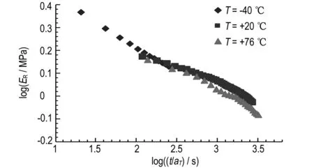
Fig.8 Shifting process using WLF method

Fig.9 Masster curve using WLF method

3.3 The Arrhenius Method

The Arrhenius relationship is verified at temperatures under the glass transition temperature of the material, and the Arrhenius TTS method for shift factor calculation is shown in Eq.7[2, 9].

(7)

whereCais the material constant that is a function of the activation energy (Ea) and the universal gas constant (R),Ca=Ea/2.303R).Tis the test temperature in K, andT0is the reference temperature (293 K). To obtain the material constant we must plot logaTverses (1/T-1/T0) and then the slop of the resulting line will be represent the material constant as shown in Fig.10, soCa=572.4. Now, the shift factors at different temperatures can be obtained as shown in Fig.11, and by using Eq.6 the master curve of the relaxation modulus according to Arrhenius method can be plotted as shown in Fig.12.

Fig.10 Linearized Arrhenius equation

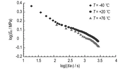
Fig.11 Shifting process using Arrhenius method

Fig.12 Master curve using Arrhenius method

4 Results and Analysis

The master curves generated based on the basic TTS method, the WLF method, and the Arrhenius method using the same experimental relaxation test data presented in Fig. 3 are plotted in Fig.13. The plots are for relaxation modulus as a function of reduced time in the log-log scale. All the curves are very similar, and this is an indication of the suitability of these methods for generating the relaxation modulus master curves of solid propellant. However, it should be stressed here that generation of satisfactory master curves and its accuracy is mostly dependent on the following factors:

Experimental test data consistency, which is a function of different variables, including both the parameters and the set-up of the relaxation test, machine vibrations or noises, specimen homogeneity and uniformity, specimen fabrication for example the dimensions and parallelism of end surfaces of the specimen, and the variation of humidity conditions.

(2)The behavior of the shift factor variation with temperature.

(3)The condition of the polymeric material state.

(4)The heating rate applied to arrive to the desired temperature.

However, the analysis of the results demonstrated that the basic method for TTS has the highest accuracy of the relaxation modulus curve fitting given determination coefficient (R2=0.9992), and this is not surprising because this method uses only the experimental data. Likewise, both the empirical methods can get acceptable results if appropriate material constants are used in these methods. Table 3 demonstrates the main statistical factors obtained during calculation of material constants, and then we can note the effect of these results on the accuracy of fitting curves. The sum of squared error (SSE), is a preliminary statistical calculation that leads to other data values. It is useful to be able to find how closely related those values are. The root mean squared error(RMSE) is the distance, on average, of a data point from the fitted line,measuring along a vertical line. It seems that the data meet WLF method givenR2coefficient (R2=0.9984), while the data meet the Arrhenius method givenR2coefficient (R2=0.9974), less than the WLF one. Compared to the other two methods, the major advantage of the basic method is that it revolves around the actual experimental data without introducing any external constant when generation the master curve, while the WLF and Arrhenius methods use already existing empirical formulas which are dependent on externally determined material constants. Table 4 is a summary of the analysis and the calculated shift factors at different temperatures when generating the master curves of solid propellant. In Fig. 14, another type of master curve can be obtained from the previous calculation shows the relation between the shift factors corresponding to each temperature. It can be observed that the data meet WLF method given higherR2coefficient, and also given lower error than the data meet the Arrhenius method. In order to simulate the nonlinear viscoelastic behavior of the composite solid propellant under different loads and conditions using various commercial finite element codes (Ansys, Abaqus, Mark, etc.), one of the time-temperature dependent shift functions must be used, and the material constants such asC1,C2, andCamust be entered as determined by the shift function specified and selected by the user in the code.

Fig.13 Master curve of AP-HTPB solid propellant obtained using the three methods

Table 3 Statistics of analysis and material constant calculation for HTPB solid propellant

parameterWLFmethodC1=-5．4 C2=770．27ArrheniusmethodCa=572．4SSE0．00052470．002355R20．99890．9932RMSE0．001560．03431

Table 4 List of analysis and calculated parameters of master curves for HTPB solid propellant

parameterbasicmethodWLFmethodArrheniusmethodaT-40℃0．4419060．4312510．485892aT+20℃111aT+76℃3．0021472．8518463．184198R20．99920．99840．9974

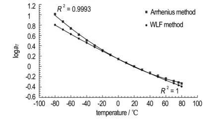
Fig.14 Shift factors corresponding to each temperature

5 Conclusions

In this paper,a series of conventional relaxation tests have been performed using a universal test machine at a broad range of temperatures (-40, +20, +76 ℃) to evaluate and get the master curves of the relaxation modulus for AP-HTPB composite solid propellant as a purpose of reduced time and at a reference temperature of 20 ℃. These master curves were generated according to three different methods (the basic, WLF, and Arrhenius) by using the TTS principle, and then comparative study was conducted to show the level of accuracy for each method. The following conclusions can be drawn:

(1)The basic method is the best method for generating a fit function for the relaxation modulus master curve followed by the WLF method and lastly, the Arrhenius method.

(2)The results presented here can be used as a reference for selecting the appropriate methods for generating the relaxation modulus master curve of AP-HTPB solid propellant.

(3)Most of the finite element software′s need some material constants to define the time-temperature dependent material method, so the basic method cannot be used alone and some material constants must be calculated using empirical formulas like WLF or Arrhenius methods, and between these two methods, the WLF method would be recommended.

[1]Bohwi S, Jaehoon K. Estimation of master curves of relaxation modulus and tensile properties for solid propellant [J].AdvancedMaterialsResearch, 2014, 871: 247-252.

[2]Salvador N, Antonio M. New method for estimating shift factors in time-temperature superposition models [J].JournalofThermalAnalysisandCalorimetry, 2013, 113: 453-460.

[3]Chyuan S. Nonlinear thermoviscoelastic analysis of solid propellant grains subjected to temperature loading [J].FiniteElementsinAnalysisandDesign, 2002, 38(7): 613-630.

[4]Chyuan S. Dynamic analysis of solid propellant grains subjected to ignition pressurization loading [J].JournalofSoundandVibration, 2003, 268(3): 465-483.

[5]Chyuan S. Studies of Poisson′s ratio variation for solid propellant grains under ignition pressure loading [J].InternationalJournalofPressureVesselsandPiping, 2003, 80(12): 871-877.

[6]Bihari B K, Waniet V S, Rao N P N, et al. Determination of activation energy of relaxation events in composite solid propellants by dynamic mechanical analysis [J].DefenseScienceJournal, 2014, 64(2): 173-178.

[7]Marimuthu R, Nageswara B. Development of efficient finite elements for structural integrity analysis of solid rocket motor propellant grains [J].InternationalJournalofPressureVesselsandPiping, 2013, 111: 131-145.

[8]Xu J, Ju Y, Han B. et al. Research on relaxation modulus of viscoelastic materials under unsteady temperature states based on TTSP [J].MechanicsofTime-DependentMaterials, 2013, 17(4) : 543-556.

[9]Lubinda F, Allex E, Geoffrey S. Evaluating and comparing different methods and models for generating relaxation modulus master-curves for asphalt mixes [J].ConstructionandBuildingMaterials, 2011, 25(5) : 2619-2626.

[10]Davenas A. Solid rocket propulsion Technology [M]. First English Edition, New York, Pergamon Press, 1993, Chapter 6.

[11]Ferry J D. Viscoelastic properties of polymers [M]. 3rd Edition, John Willy and Sons, 1980.

[12]Zheng Z, Zhang R. Implementation of viscoelastic material model to simulate relaxation in glass transition [C]∥Excerpt from the Proceedings of the 2014 COMSOL Conference in Boston, 2014.

[13]Carlrton J M. SRM propellant and polymer materials structural test program. NASA Technical Paper 2821, 1988.

[14]KGNC A, Burgoyne C J. Time-temperature superposition to determine the stress-rupture of aramid fibres [J].AppliedCompositeMaterials, July 2006, 13(4) : 249-264.

[15]ROBERT F L. Viscoelastic properties of rubberlike composite propellants and filled elastomers [J].ARSJournal, 2015, 31(5): 599-608.