Spatial relationship between energy dissipation and vortex tubes in channel flow*

Lie-kai Cao (曹列凯), Dan-xun Li (李丹勋), Huai Chen (陈槐), Chun-jing Liu (刘春晶)

1.State Key Laboratory of Hydroscience and Engineering, Tsinghua University, Beijing 100084, China, E-mail:clk_THU@hotmail.com

2.State Key Laboratory of Hydrology-Water Resources and Hydraulic Engineering, Nanjing Hydraulic Research Institute, Nanjing 210029, China

3.State Key Laboratory of Simulation and Regulation of Water Cycle in River Basin, China Institute of Water Resource and Hydraulic Research, Beijing 100038, China

Spatial relationship between energy dissipation and vortex tubes in channel flow*

Lie-kai Cao (曹列凯)1, Dan-xun Li (李丹勋)1, Huai Chen (陈槐)2, Chun-jing Liu (刘春晶)3

1.State Key Laboratory of Hydroscience and Engineering, Tsinghua University, Beijing 100084, China, E-mail:clk_THU@hotmail.com

2.State Key Laboratory of Hydrology-Water Resources and Hydraulic Engineering, Nanjing Hydraulic Research Institute, Nanjing 210029, China

3.State Key Laboratory of Simulation and Regulation of Water Cycle in River Basin, China Institute of Water Resource and Hydraulic Research, Beijing 100038, China

The spatial relationship between the energy dissipation slabs and the vortex tubes is investigated based on the direct numerical simulation (DNS) of the channel flow. The spatial distance between these two structures is found to be slightly greater than the vortex radius. Comparison of the core areas of the vortex tubes and the dissipation slabs gives a mean ratio of 0.16 for the mean swirling strength and that of 2.89 for the mean dissipation rate. These results verify that in the channel flow the slabs of intense dissipation and the vortex tubes do not coincide in space. Rather they appear in pairs offset with a mean separation of approximately 10η.

Energy dissipation, vortex, channel flow, swirling strength, turbulent structure

Introduction

The structure of the intermediate and fine scales of the turbulent shear flows remains one of the most challenging issues in the turbulence research. Understanding the dynamics of these scales is essential for an accurate statistical description and the numerical simulation of the turbulent shear flows.

The energy dissipative structures, characterized by the Kolmogorov scaleη, represent the finest eddies in the turbulence. The kinetic energy dissipation is generally complex, involving sheet-, line- and blob-like structures[1]. The intense energy dissipation structures (defined as a region over which the magnitude of energy dissipation is much larger than the global mean value), however, tend to be more slab-like, as has been identified in various experimental studies[1,2]. The dissipation slab possesses a charac-teristic thickness of 5η-10ηand a length of 50η-100ηin the order of magnitude[1,2].

Vortex structures are comparable in size to the dissipative structures. Vortex cores correspond to the most intense realizations of the background vorticity, and they tend to form tube-like structures, as identified in various kinds of turbulent flows, e.g., the isotropic turbulence[3], the turbulent jet[1,4], the pipe flow[5], the channel flow[6], and the turbulent boundary layers[7]. Herpin et al.[8]found that the core diameter of the vortex tubes was nominally 8η, and Ganapathisubramni et al.[1]reported similar results of 6ηto 15η. The typical length of the vortex tubes was found to be approximately 60η-100η[1].

The relationship between the vortex structures and the dissipative structures is a research focus. Results obtained based on the DNS concluded that intense dissipative structures occur in the vicinity of intense vortex cores[3,9]. The measurements of previous studies[1,10,11]reported similar conclusions that the dissipation structures and the vortices are spatially and temporally separated. In particular, Zeff et al.[10]studied conditional averages of the growth rate of the dissipation, finding that the dissipation decreases whenthe centre of a vortex tube is approached. Ganapathisubramani et al.[1]computed the joint probability density function (PDF) between the swirling strength and the energy dissipation rate to investigate the concurrence of intense values of the two quantities, showing that an intense dissipation is not coincident with an intense swirling strength. Fiscaletti et al.[11]estimated the distance between the vortex structure and the intense dissipation structure by a cross correlation of the swirling strength and the dissipation rate, which is found to be comparable to the radius of the vortex.

Table 1 Parameters of the DNS data from Del Alamo et al.[13]

Table 2 Interpolated planes from the DNS dataset

Regarding the energy dissipation field associated with the vortex tubes, most results indicate that the two structures are separated, and the peaks of the dissipation rate are at the periphery of the vortex tubes. These results are mainly based on the analysis of the isotropic turbulent flow and the turbulent jet, and without much work on the analysis of channel flows. Moreover, some contradictory evidence exists, for example, Pirozzoli[12]reported that the energy dissipation peaks are found at the vortex centre rather than around the periphery.

In the present study we analyze the dissipation fields associated with the vortex tubes using a direct numerical simulation (DNS) database of channel flows. The main objective is to perform both qualitative and quantitative analyses to reveal the spatial relationship between the intense dissipation structures and the vortex tubes in channel flows.

1. Methodology

1.1 DNS data

The analysis is based on a DNS database of the turbulent channel flows by Del Alamo et al.[13]. The original datasets include two series of simulations: in the first one, large numerical boxes are used to account for large-scale energetic structures, and in the second one, smaller boxes are used to increase the Reynolds number. The L950 case from the first series is selected and introduced briefly here. Detailed information can be found in Del Alamo et al.[13].

The friction Reynolds number of the flow iswhereuτis the wall friction velocity andνis the viscosity. The simulation covers a spatial domain ofandalongx(steamwise),y(wall-normal) andz(spanwise) directions, respectively, wherehis the channel half-width. The domain is discretized into an array of 3072(x)×385(y)×2304(z) points. In the present analysis, we compute statistics related with a part of the domain with a volume of 16πh/3(x)×1h(y)×2πh(z), corresponding to an array of 2 048(x)×193(y)×1536(z) points. It is worth noting that the original discretization is based on uniform spatial resolutions inxandzdirections (the flow homogeneity is assumed in these two directions) and non-uniform resolution inydirection (finer grids are used in the near-wall region in order to better resolve the velocity gradient).

For each mesh, three instantaneous velocity components and nine corresponding velocity gradients are considered. Major parameters of the DNS database are summarized in Table 1.

To facilitate the vortex detection and analysis, the native 2-D velocity fields inXYandYZplanes are interpolated on regular meshes using the bi-cubic spline interpolation technique, as by Herpin et al.[14]. Different spacings inydirection are used inXYandYZplanes, i.e., Δy+=7.5 (similar to Δx+) inXYplane and Δy+=3.8 (equal to Δz+) inYZplane. The original uniform resolution inXZplane is maintained (Δx+=7.6and Δz+=3.8). Then the 3-D velocity fields are projected into the coordinate planes, with a separation distance of+38 inzdirection and of+76 inxdirection. For each sliced plane, a total number of 30 instantaneous velocity fields, uncorrelated in time, are used for statistical analysis. In total, we have extracted 153×30XYplanes, 204×30YZplanes, and 193×30XZplanes for further analysis, and there are 2048×124, 245×1536 and 2048×1536 grid points inXY,YZandXZplanes, respectively. The characteristics of the interpolatedXYandYZplanes as well as the nativeXZplanes are summarized in Table 2.

1.2 Vortex identification

Vortices can be extracted from the background turbulence through various point-wise methods that involve kinematic parameters derived from the velocity gradient tensor ∇u[15]. In the present study we use the swirling strength method. This method, first proposed by Zhou et al.[15], takes the imaginary part of the complex eigenvalues,λci, as the vortex indicator.

To eliminate the wall-normal dependence ofλciin the wall-bounded flows, similar to the normalisation methods in the previous research[16], we recommend to use the normalisation ofλciwith its local root mean square (rms)

whereis the rms ofλciat a givenyposition. A comparison of PDFs of(whereandΛatand 0.9 indicates that the wall-normal dependence ofciλis successfully eliminated after the normalisation (Fig.1). Following Wu and Christensen[16], Herpin et al.[14], Chen et al.[17]and Zhong et al.[18], we useΛsto identify and visualize the vortices in the present study. It is worth noting that the use of other vortex detection functions does not alter the results as these methods are essentially equivalent.

To extract vortexes from a background turbulence, a non-zero threshold has to be used such that

Fig.1 Comparison of probability density functions inXZplane for different values of

There is no general consensus on the selection of an appropriate non-zero threshold in the literature[1,6,14-17]. Zhou et al.[15]determinedαas a percentage of the maximumΛssuch that

Zhou et al.[15]recommended =12%-20%βbased on their findings that the extracted vortices have varying sizes but a similar shape at such a threshold. In order to extract intense vortex tubes, we use a threshold ofα=2 at whichβis equal to about 13%, similar to the lower limit given by Zhou et al.[15]. This threshold is greater than that used by Wu and Christensen, whereα=1.5[16].

The vortex radius is calculated by using the algorithm proposed by Gao et al.[6].

1.3 Energy dissipation slab

The dissipation rate of the kinetic energy per unit volume,ε, is calculated by using nine velocity gradient components. The volume-averaged and plane-averaged (XZplane) energy dissipation rates, 0εandεp, are quantified by averaging over the entire domain and theXZplane, respectively. Further analysis of the energy dissipation rate in a channel flow is performed by computing the cumulative distribution functions (CDFs).

Fig.2 Comparison of probability density functions ofεandEinXZplane for various values ofy/h

Instantaneous dissipation slabs can be extracted based on the iso-surfaces of the dissipation rate. Similar to the swirling strength, the dissipation rate also exhibits a wall-normal dependence (Fig.2(a)). This wall-normal dependence makes it difficult to select a universal threshold, i.e., a proper threshold for showing inner-layer dissipation structures may lead to“blurring” in the outer layer, and conversely, raising the threshold to “accommodate” the outer-layer dissipation structures may result in “cluttering” of those in the inner layer. By analogy to the normalisation procedure used for the vortex identification, we normalize the dissipation rate with its plane-averaged value to eliminate the wall-normal dependence (Fig.2(b))

whereis the plane-averaged dissipation rate in the plane aty.

The normalisation of Eq.(4) yields a value ofEwith a negligible wall-normal dependence, based on which the energy dissipation structures can be extracted through similar procedures used for the vortex identification. A threshold ofE=3 is selected (corresponding to 90% of the points of the cumulative distribution function inXZplane), that is, the intense dissipation regions in the flow field are identified asε≥3εp. This threshold is also used by Fiscaletti et al.[11]to extract a high dissipation structure.

1.4 Spatial relationship analysis

The spatial relationship between the energy dissipation and the vortex structures is investigated through three approaches in the present analysis.

The first approach is to project the instantaneous iso-surfaces ofΛsandEinto a slicedXYplane or into the 3-D domain. This approach is easy to implement, and can provide important intuitive information.

Fig.3 (Color online) Schematic diagram of the conditional average approach (green points denote vortex cores)

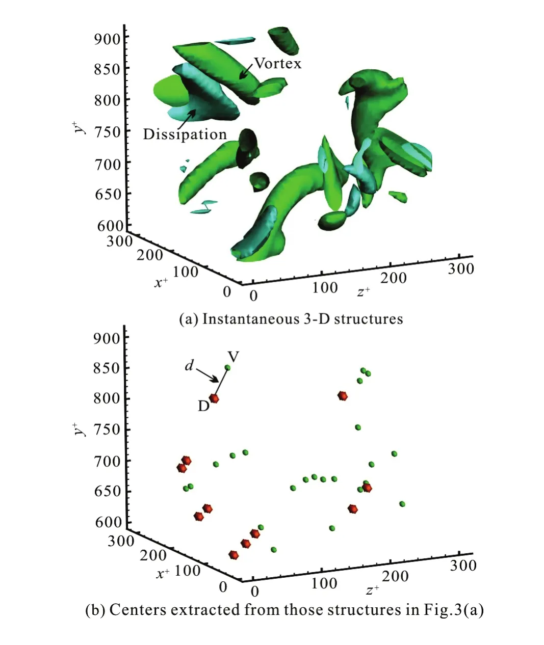
Fig.4 (Color online) Centers extracted from instantaneous 3-D structures of dissipation and vortices

The second approach involves a conditional average in variousXYplanes at+=2 006zto examine the energy dissipation in the vicinity of vortex centers. This approach consists of four steps. Firstly, all points ofΛs＞2 are identified, and their local maxima are marked as the vortex cores in theXYplane. Secondly, each vortex is characterized by a rectangular region of 40×40 mesh. Thirdly, an ensemble is established by collecting all these rectangular vortex regions with samey+in the time series (as those vortices in the stripe with grey background color in Fig.3). Lastly, the swirling strength and the energy dissipation rate are statistically averaged to obtain the final results.

The third approach makes use of the quantification of the spatial distances between vortex tubes and their neighboring energy dissipation structures. The centres of the instantaneous 3-D structures of dissipation and the vortices are identified as the local maxima in the vortex tubes and the dissipation slabs, as shown in Fig.4. Once the vortex centreand its neighboring dissipation centreare obtained, the distance between them can be readily calculated

The ratios ofλcias well asεbetween the two cores are defined as

whereλciDandλciVare the swirling strengths at the dissipation centre and at the vortex centre, respectively,εDandεVare similarly defined.

Fig.5 Distribution of plane-averaged energy dissipation along

Fig.6 Cumulative distribution functions of the dissipation rate

2. Results

2.1 Energy dissipation

The volume-averaged energy dissipation rateε0over the entire 3-D domain is 0.011 m2s-3. The normalized plane-averaged dissipation ratein theXZplane is shown in Fig.5. A relatively constantεpis observed in the vicinity of the channel bed+(y＜8) followed by a steady decrease with increasing+y. This finding is consistent with the results of Herpin et al.[14]. Compared withε0,εpis greater in the region ofy+＜23 due to the contribution of the mean shear. to 72% in the outer layer (y+=700) and 61% in the viscous sublayer+(y=5). These results are consistent with those obtained by Ganapathisubramani et al.[1].

The instantaneous 3-D dissipative structures are visualized through iso-surfaces of the the normalized dissipation rate,E. As shown in Fig.7, most dissipative structures are slab-like of a finite thickness. These structures are named the “dissipation sheet” by Ganapathisubramani et al.[1].

Fig.7 (Color online) Two typical iso-surfaces of instantaneous dissipation structures forE=3

Fig.8 Distribution of the scaled Kolmogorov length scale

The CDFs of the dissipation rate in the 3-D domain and the three orthogonal planes are shown in Figs.6(a)-6(d), respectively. In the 3-D domain, about 86% of the energy dissipation rate is less than the volume-averagedε0(Fig.5(a)). Similar percentages are observed in differentXYplanes (corresponding toz+=200, 470, 2 000 and 7 000 in Fig.6(b)) and differentYZplanes (corresponding tox+=49, 298, 1 009 and 2 006 in Fig.6(c)). InXZplanes (Fig.6(d)), the CDF profiles display a visible wall-normal dependence, and the percentage reduces

Fig.9 (Color online) Typical instantaneous vortex structures visualized withΛs=2

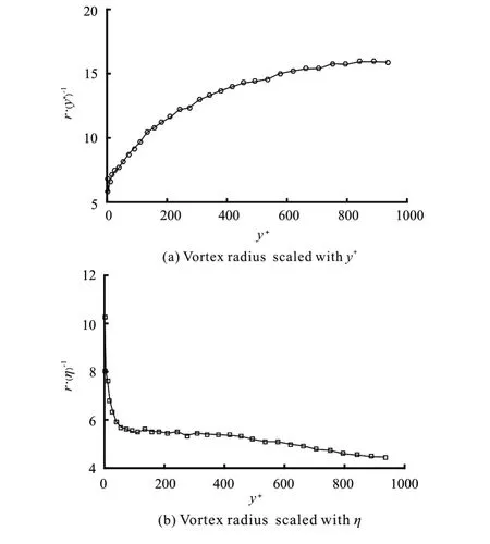
Fig.10 Mean vortex radius scaled with+yandη

Fig.11 (Color online) Color maps of swirling strength and energy dissipation rate in the slicedXYplane at+=2 006z

Figure 8 presents the scaled Kolmogorov length scaleη/y*alongy+in which. It is clear thatremains roughly constant in the nearwall regionand then turns to increase steadily withy+. Herpin et al.[14]reported similar results.

2.2 Vortex characteristics

The tube-like vortex structures are visualized through the contours ofΛs. Figure 9 shows typical iso-surfaces forΛs=2. It is clearly visible that the channel flow is also prominent with vortex tubes.

The mean radius of the tube-like vortices displays a visible wall-normal dependence, as shown in Fig.10. When scaled withy*, the mean radius increases with+y, when scaled with localη, however, it decreases with+y. These trends agree well with the previous results[19]. In the outer layer, a similar magnitude ofris observed as those obtained by Ganapathisbramani et al.[1], and Pirozzoli[12]. The magnitude ofr+(whereis smaller than those reported by Gao et al.[6], and such a disagreement is possibly due to different thresholds used.

2.3 Spatial relationship between dissipation slabs and vortices

Fig.12 (Color online) Overlay iso-surfaces of swirling strength forΛs=2 and energy dissipation rate forE=3

Figure 11 presents a typical 2-D instantaneous velocity field in theXYplane at+=2 600zto illustrate the spatial relationship between the dissipation slabs and the vortex structures. The distributions ofΛsandEindicate that both the vortices and the intense dissipation regions are locally concentrated (Figs.11(a), 11(b)). These local patterns are better illustrated through a binary thresholding withΛs=2 andE=3, respectively (Figs.11(c), 11(d)). In the same plot, the distributions ofΛsandEshow clearly that the intense dissipation slabs are located in the vicinity of multiple nested vortex tubes (Fig.11(e)). Similar results are obtained in otherXYplanes andXZandYZplanes.

Figure 12 presents a typical instantaneous 3-D iso-surfaces ofΛsandE. In the region of300, both the vortex tubes and the intense dissipation structures are densely distributed, in the region ofthose structures become sparse. It is clearly visible that the elongated vortex tubes are surrounded by intense dissipation slabs. This observation is consistent with the previous studies[1,3,9].

Figure 13 presents the conditionally averaged results forand 700. Similar procedures of the binary thresholding and the superposition are used in plotting the figure. Again, it is clearly visible that the intense vortices and the intense dissipation structures do not collapse in space. Note that the spatial relationship between these two kinds of structures seem to be related toi.e., the vortices and the dissipation structures seem to stand shoulder by shoulder aty+=74 whereas the vortices are surrounded by the dissipation structures aty+=700.

The results of the distance between the vortex tubes and the dissipation slabs are presented in Table 3. The mean distance is, about twice the radius of the vortex tube. This fact supports the previous findings that the intense dissipation structures are generally distributed in the vicinity of the vortex tubes. The mean values ofMλandMεareandrespectively, indicating that the vortex cores and the dissipation structures do not collapse in space.

Figure 14 shows the CDFs of the distanced. About 80% of the values ofdfall in the interval of (10y*-40y*), and their median is at 28y*, about twice of the vortex radius.

Figure 15 shows the plane-averaged distancedswith respect toy+. In the inner layer,increases with the increase of+y, but in the outer layer the trend reverses (Fig.15(a)). In the outer layer, the magnitude ofdsvaries in the range of 7η-10η(Fig.15(b)), about twice the radius of vortex tubes calculated as in the range of 4η-6η. The spatial distance is similar to the estimation of 9ηbyFiscaletti et al.[11]and to the distance in the range of 8η-12ηin a Burgers vortex model.

Figure 16(a) shows the plane-averagedMsλas a function of the wall-normal position. It is apparent that fory+＞50,Msλremains close to 0.16 with a negligible wall-normal dependence. Figure 16(b) shows that in the outer layer, the probability ofMλ=0 fluctuates around 59.5%, indicating that about 60% of the intense dissipation slabs are located in the non-vortex region. These results further verify that the cores of the intense dissipation structures and the vortex tubes are not overlapped in space.

3. Discussions

As both the vortex tubes and the energy dissipation slabs are complex spatial structures, it is difficult, if not impossible, to accurately define and quantify the distances between them. In order to get comparable results, the present study follows the commonly used definitions and methods.

When a dissipation slab is immediately close to a vortex tube (Fig.17), the distance between these two structures can be defined as

Fig.13 (Color online) Color maps of conditional averaged swirling strength and dissipation rate aty+=74 and+=700y

Fig.14 CDFs of distance in the whole domain

whereφandHrepresent the vortex diameter and the thickness of the intense dissipation structure, respectively. Previous studies reveal thatH=6η-12η[1-2]. The present study indicates thatφ=8η-12η. Based on these results, one may haveL=6η-12ηsimilar to the calculated values (7η-10η).

Pirozzoli[12]reported that the maximum dissipation occurs in the vortex centre rather than around the periphery. His observation may be closely related to his average procedure (azimuthally averaging the energy dissipation around vortex tubes), not necessarily related to the true physics. For illustration, we also make a spatial average analysis of the energy dissipation rate along the radial direction. Figure 18 presents the result aty+=700 (based on the data from the averaged results in Section 3.3). Similar to the finding of Pirozzoli[12], a distinct peak occurs at the centre of the vortex and a secondary peak occurs near the edge of the vortex. This trend can be explained by the non-circular characteristics of the dissipative struc-tures in a sliced plane (for instance, see Fig.13). For an individual vortex, the dissipation rate in the vortex core is always smaller than that in the outer edge. However, due to the fact that the dissipation structure typically does not surround the vortex as a circle, the averaging over the area equidistant to the vortex core may result in the pattern shown in Fig.18.

Fig.15 Mean distance ofdsscaled withy*andη

Fig.16 Plane-averagedMsλand the probability ofM=0λ Mλ=0 along+y

Fig.17 (Color online) Schematic diagram of a neighboring pair of dissipation slab and vortex tube

Fig.18 Radial distribution of energy dissipation.εrmeans the averaged dissipation rate at a givenr

4. Conclusions

Based on the DNS data of the turbulent channel flow, the spatial distributions of intense dissipation slabs and vortex tubes are investigated. Major findings are as follows:

(1) A relatively uniform distribution of the energy dissipation is observed in theXZplane, uneven distributions are observed in bothXYandYZplanes, i.e., the plane-averaged dissipation rate decreases with the increase of+y. In more than 86% of the flow region, the dissipation rate is below the average value.

(2) The typical instantaneous velocity fields reveal that the vortices are organized in tube-like structures and the intense dissipation structures are slab-like with a finite thickness. Intense dissipation slabs are found in the vicinity of vortex tubes.

(3) The mean distances between the neighboring vortex tubes and the dissipation slabs are found to be approximately equal to 28.1y*, slightly larger than the vortex radius. Scaled with the Kolmogorov scale, the distance varies in the range of 7η-10η.

(4) Comparison of the core areas of the vortex and the dissipation slab gives a mean ratio of 0.16 for the mean swirling strength and that of 2.89 for the mean dissipation rate. This further verifies that the regions of the intense dissipation do not collapse to those of the vortex tubes.

[1] Ganapathisubramani B., Lakshminarasimhan K., Clemens N. T. Investigation of three-dimensional structure of fine scales in a turbulent jet by using cinematographic stereoscopic particle image velocimetry [J].Journal of Fluid Mechanics, 2008, 598: 141-175.

[2] Tsurikov M. S., Clemens N. T. The structure of dissipative scales in axisymmetric turbulent gas-phase jets [C].AIAA 40th Aerospace Sciences Meeting. Reno, Nevada, 2002.

[3] Vincent A., Meneguzzi M. The dynamics of vorticity tubes in homogeneous turbulence [J].Journal of Fluid Mechanics, 1994, 258: 245-254.

[4] Violato D., Scarano F. Three-dimensional vortex analysis and aeroacoustic source characterization of jet core breakdown [J].Physics of Fluids, 2013, 25(1): 015-112.

[5] Mouri H., Hori A., Kawashima Y. Laboratory experiments for intense vortical structures in turbulence velocity fields [J].Physics of Fluids, 2007, 19(5): 055-101.

[6] Gao Q., Ortiz-Dunnas C., Longmire E. K. Analysis ofvortex populations in turbulent wall-bounded flows [J].Journal of Fluid Mechanics, 2011, 678: 87-123.

[7] Elsinga G. E., Adrian R. J., Van Oudheusden B. W. et al. Three-dimensional vortex organization in a high-Reynolds-number supersonic turbulent boundary layer [J].Journal of Fluid Mechanics, 2010, 644: 35-60.

[8] Herpin S., Stanislas M., Foucaut J. M. et al. Influence of the Reynolds number on the vortical structures in the logarithmic region of turbulent boundary layers [J].Journal of Fluid Mechanics, 2013, 716: 5-50.

[9] Kaneda Y., Ishihara T. High-resolution direct numerical simulation of turbulence [J].Journal of Turbulence, 2006, 7: 1-17.

[10] Zeff B. W., Lanterman D. D., McAllister R. et al. Measuring intense rotation and dissipation in turbulent flows [J].Nature, 2003, 421(6919): 146-149.

[11] Fiscaletti D., Westerweel J., Elsinga G. E. Long-range mu-PIV to resolve the small scales in a jet at high Reynolds number [J].Experiments in Fluids, 2014, 55: 1812.

[12] Pirozzoli S. On the velocity and dissipation signature of vortex tubes in isotropic turbulence [J].Physica D: Nonlinear Phenomena, 2012, 241(3): 202-207.

[13] Del Alamo J. C., Jimenez J., Zandonade P. et al. Scaling of the energy spectra of turbulent channels [J].Journal of Fluid Mechanics, 2004, 500: 135-144.

[14] Herpin S., Stanislas M., Soria J. The organization of near-wall turbulence: a comparison between boundary layer SPIV data and channel flow DNS data [J].Journal of Turbulence, 2010, 11: 1-30.

[15] Zhou J., Adrian R. J., Balachandar S. et al. Mechanisms for generating coherent packets of hairpin vortices in channel flow [J].Journal of Fluid Mechanics, 1999, 387: 353-396.

[16] Wu Y., Christensen K. T. Population trends of spanwise vortices in wall turbulence [J].Journal of Fluid Mechanics, 2006, 568: 55-76.

[17] Chen Q., Zhong Q., Wang X. et al. An improved swirling-strength criterion for identifying spanwise vortices in wall turbulence [J].Journal of Turbulence, 2014, 15(2): 71-87.

[18] Zhong Q., Li D., Chen Q. et al. Coherent structures and their interactions in smooth open channel flows [J].Environmental Fluid Mechanics, 2015, 15(3): 653-672.

[19] Pirozzoli S., Bernardini M., Grasso F. Characterization of coherent vortical structures in a supersonic turbulent boundary layer [J].Journal of Fluid Mechanics, 2008, 613: 205-231.

(Received July 11, 2015, Revised October 21, 2015)

* Project supported by the National Natural Science Foundation of China (Grant No. 51127006).

Biography:Lie-kai Cao (1990-), Male, Ph. D. Candidate

Chun-jing Liu,

E-mail: liucj@iwhr.com