
An Effcient Numerical Solution of Nonlinear Hunter–Saxton Equation
2018-01-24 06:22KouroshParandandMehdiDelkhoshDepartmentofComputerSciencesShahidBeheshtiUniversityTehranIran
Kourosh Parandand Mehdi DelkhoshDepartment of Computer Sciences,Shahid Beheshti University,G.C.,Tehran,Iran
2Department of Cognitive Modelling,Institute for Cognitive and Brain Sciences,Shahid Beheshti University,G.C.,Tehran,Iran
Nomenclature
u(x,t) unknown function t time position coordinate u¯(x,t) the approximate solution x scaled coordinate ηFTnαbasis functionΦ(t)the vector of basis functions α the order of basis functionsηlength of the domain of function definition A unknown coeffcients vector K unknown coeffcients matrix m the number of basis functions E the maximum of the absolute error
1 Introduction
The nonlinear Hunter–Saxton equation is one of the partial differential equations that by some researchers is studied:
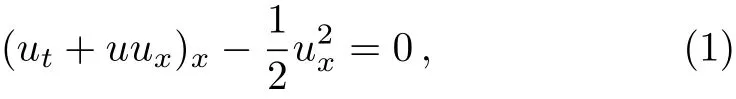
wheretandxare time position and scaled coordinates,respectively.The structures of the problem,for the first time,are described by Hunter and Saxton in 1991 in their paper entitle “Dynamics of Director Fields”.[1]They have used this equation for studying a nonlinear instability in the direct field of a nematic liquid crystal,and have shown that smooth solutions of the asymptotic equation break down in finite time.
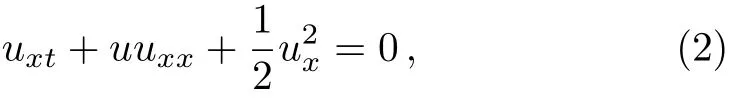
The Hunter–Saxton equation also arises as the shortwave limit of the Camassa–Holm equation,[2]an integrable model the unidirectional propagation of shallow water waves over a flat bottom,[3]and the geodesic flow on the diffeomorphism group of the circle with a bi-Hamiltonian structure,[4]which is completely integrable.[5]
or,equivalently,
Because of the many applications of this equation has been studied by some researchers,such as Beals et al.[6]have obtained the inverse scattering solutions to this equation,Penskoi[7]has studied Lagrangian timediscretizations of the Hunter-Saxton equation by using the Moser–Veselov approach,Yin[8]has proved the local existence of strong solutions of the periodic Hunter–Saxton equation and has shown that all strong solutions except space-independent solutions blow up in finite time,Lenells[9]has considered the Hunter–Saxton equation models the geodesic flow on a spherical manifold,Xu and Shu[10]have used the development of the local discontinuous Galerkin method and a new dissipative discontinuous Galerkin method for this equation,Wei and Yin[11]have considered the periodic Hunter–Saxton equation with weak dissipation,Wei[12]has obtained global weak solution for a periodic generalized Hunter–Saxton equation,Nadja fikhah and Ahangari[13]have studied a Lie group symmetry analysis of the equation and have obtained some exact solutions,Baxter et al.[14]have obtained the separable solutions and self-similar solutions of the equation,Arbabi et al.[15]have obtained a semi-analytical solution for the equation using the Haar wavelet quasilinearization method.
We know that,the solution of some equations is generated by fractional powers or the structure of the solution of some equations is not exactly known.For example,one of the famous equations that its solution is generated by fractional powers is Thomas-Fermi equation.[16−17]Baker[17]has proved that the solution of Thomas–Fermi equation is generated by the powers oft1/2.For these reasons,in this paper,we decided that we solve the Hunter–Saxton equation using the fractional basis,namely the bivariate generalized fractional order of the Chebyshev function(BGFCF),in order to obtain more information about the structure of the solution and obtaining acceptable results.
The B-GFCFs are introduced as a new basis for Spectral methods and this basis can be used to develop a framework or theory in Spectral methods.In this research,the fractional basis was used for solving a partial differential equation(Hunter–Saxton equation)and it provided insight into an important issue.The B-GFCF collocation method is combined with the quasilinearization method(QLM)to calculate a more accurate and faster result.
The organization of the paper is expressed as follows:in Sec.2,the generalized fractional order of the Chebyshev functions(GFCFs)and their properties are expressed.In Sec.3,the work method is explained.In Sec.4,the numerical examples are presented to show the effciency of the method.Finally,a conclusion is provided.
2 Generalized Fractional Order of the Chebyshev Functions
The Chebyshev polynomials have many properties,for example orthogonal,recursive,simple real roots,complete in the space of polynomials.For these reasons,many authors have used these functions in their works.[18−21]
Using some transformations,some researchers extended Chebyshev polynomials to in finite or semi-in finite domains.For example,by usingx=(t−L)/(t+L),L>0 the rational Chebyshev functions on semi-in finite interval,[22−25]by usingthe rational Chebyshev functions on in finite interval,[26]and by usingx=1− 2(t/η)α,α,η>0 the generalized fractional order of the Chebyshev functions(GFCF)on the finite interval[0,η][27]are introduced.
In the present work,the transformationx=1−2(t/η)α,α,η>0 on the Chebyshev polynomials of the first kind is used,that was introduced in Ref.[27]and can use to solve differential equations.
The GFCFs are defined on the interval[0,η]and are denoted by
The analytical form of of degreenαis given by[27]
where

The GFCFs are orthogonal with respect to the weight functionon the interval(0,η):
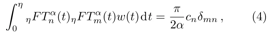
whereδmnis Kronecker delta,c0=2,andcn=1 forn≥1.
Any function of continuous and differentiabley(t),t∈ [0,η]can be expanded as follows:
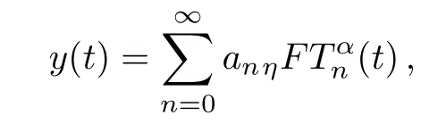
and using the property of orthogonality in the GFCFs:
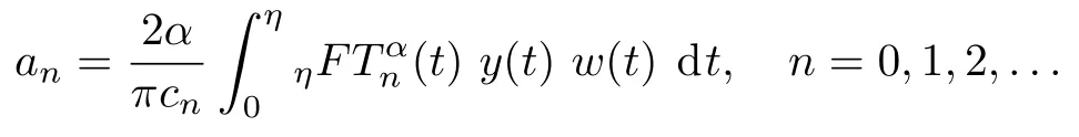
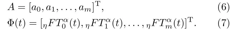
But in the numerical methods,we have to use first(m+1)-terms of the GFCFs and approximatey(t):
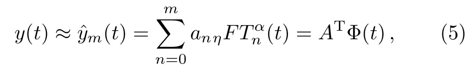
with
The following theorem shows that by increasingm,the approximation solutionfm(t)is convergent tof(t)exponentially.
Theorem1Suppose thatDkαf(t) ∈C[0,η]fork=0,1,...,m,andis the subspace generated byIffm(t)=ATΦ(t)(in Eq.(5))is the best approximation tof(t)fromthen the error bound is presented as follows
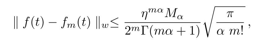
whereMα≥ |Dmαf(t)|,t∈ [0,η].
ProofSee Ref.[27].∗
Theorem 2The generalized fractional order of the Chebyshev functionhas preciselynreal zeros on interval(0,η)in the form
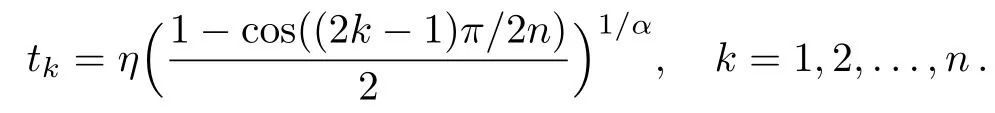
Moreover,(d/dt)ηhas preciselyn−1 real zeros on interval(0,η)in the following points:

ProofSee Ref.[27].∗
3 Methodology
In this section,the quasi-linearization method is introduced and is used for solving nonlinear Hunter–Saxton equation.
3.1 The Quasilinearization Method
The quasi-linearization method(QLM),based on the Newton–Raphson method,[28−29]by Bellman and Kalaba have introduced.[30]This method is used for solving the nonlinear differential equations(NDEs)ofn-th order inpdimensions.In this method,the NDEs convert to a sequence of linear differential equations,and the solution of this sequence of linear differential equations is convergence to the solution of the NDEs.[31−33]Some researchers have used this method in their papers.[34−37]
Occasionally the linear differential equation that gets from the QLM at each iteration does not solve analytically.Hence we can use the Spectral methods to approximate the solution.
We consider nonlinear PDEs of the form
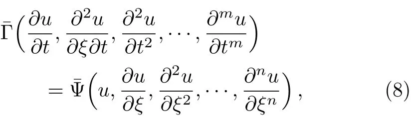
wherenandmare the orders of differentiation forξandt,respectively,t∈ [0,T],ξ∈ [a,b],u(ξ,t)is the unknown function,¯Ψ is a nonlinear operator that contains all the partial derivatives ofu(ξ,t)toξ,and¯Γ is a linear operator of both variablesξandtthat contains all the partial derivatives ofu(ξ,t)tot.
By using the transformationξ=[(b−a)/η]x+a,the intervalξ∈[a,b]can be converted into the intervalx∈ [0,η],thus Eq.(8)can be written as follows
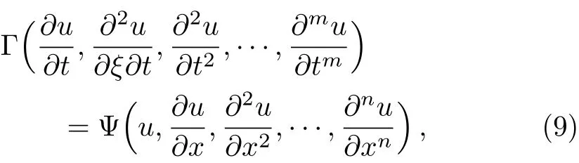
whereTandηare real positive constants,Γ =
Before applying the QLM,the operator Ψ is split into its linear and nonlinear parts and rewrite Eq.(9)as follows:
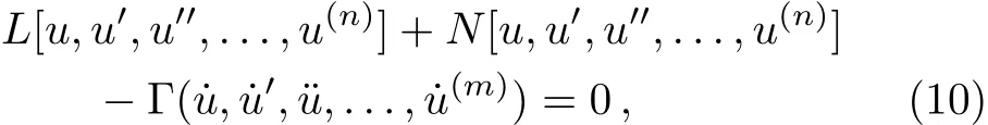
where the dots and primes denote the derivative with respect totandx,respectively,andLandNare the linear and nonlinear operators of Ψ,respectively.
Now,the QLM is used for the nonlinear operatorNas follows(similar to Taylor’s series):[38]
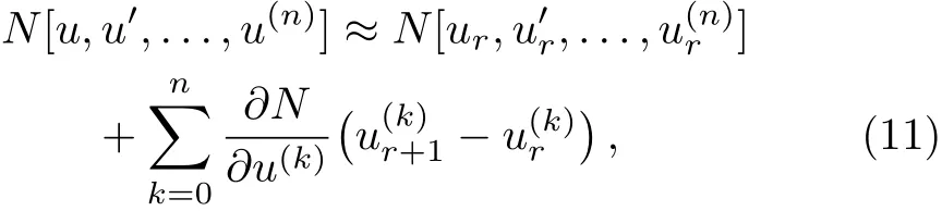
whererandr+1 denote previous and current iterations,respectively,and the functions∂N/∂u(k)are functional derivatives with respect tou(k)from theN[u,u′,...,u(n)].
By substituting Eq.(11)into Eq.(10),and using the QLM,we have

where
By using the QLM,the solution of Eq.(9)determines the(r+1)-th iterative approximationur+1(x,t)as a solution of the linear partial differential equation(12)with their initial and boundary conditions.
The QLM iteration requires an initialization or“initial guess”u0(x,t),that it is usually selected based on the initial and boundary conditions.
3.2 The B-GFCFs Collocation Method
It is assumed that the solution can be approximated by using the bivariate generalized fractional order of the Chebyshev functions(B-GFCFs)in the form

wherem1is the number of collocation points in thetspace andm2is the number of collocation points in thexspace.Equation(13)can be written in the following matrix form:

We apply the B-GFCFs collocation method to solve the linear partial differential equations at each iteration Eq.(12)with their initial and boundary conditions.
We assume thatu(x,0)=f(x)is an initial condition for Eq.(9).For satisfying the initial condition at each iteration,we define the approximate solution as follows

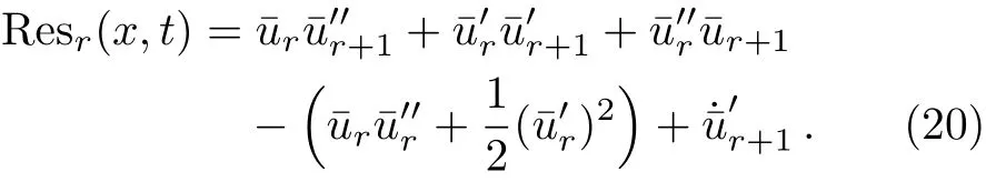
Now,to apply the collocation method,the residual function for Eq.(12)at each iteration is constructed by substituting¯ur+1forur+1:

Now,by choice(m1+1)arbitrary points{xi},i=1,...,m1+1 in the interval[0,η],and(m2+1)arbitrary points{tj},j=1,...,m2+1 in the interval[0,T]as collocation points and substituting them in Resr(x,t),and the use of their initial and boundary conditions,a set of(m1+1)(m2+1)linear algebraic equations is generated as follows(Collocation method)

By solving this system using a suitable method such as Newton’s method,the approximate solution of Eq.(9)according to Eqs.(13)and(15)is obtained.
In this study,the roots of the GFCFs in the intervals of[0,T]and[0,η](Theorem 2)have been used as collocation points in thetandxspaces,respectively.Also consider that all of the computations have been done by Maple 2015.
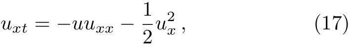
3.3 Solving Nonlinear Hunter–Saxton Equation
We consider nonlinear Hunter–Saxton equation:
with the initial and boundary conditions
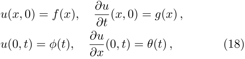
where the functionsf(x),g(x),ϕ(t),andθ(t)are suff-ciently smooth.
By applying the technique described in the previous section,we have

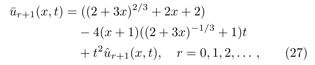
For satisfying the initial conditions at each iteration,the approximate solution¯ur(x,t)is defined as follows
and according to Eq.(16),we have
A set of(m1+1)(m2+1)linear algebraic equations is generated as follows:

By using the initial and boundary conditions(18),for satisfying the initial conditions at the first,it is assumed that the initial guessu0(x,t)=f(x)+tg(x),and the boundary conditions are implemented in the first and last rows(i.e.i=1 andi=m1+1)in Eqs.(21).By solving the linear algebraic equations,the approximate solution of Eq.(17)according to Eqs.(13)and(19)is obtained.
Now,we must try to select an appropriate value for the parameter ofα.To achieve this goal,we can use the maximum of the absolute error or the residual error.That is,we will solve the problem for various values ofα,and then based on the maximum of the absolute error or the residual error,an appropriate value forαis selected.
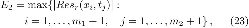
We define the maximum of the absolute error and the maximum of the residual error as follows
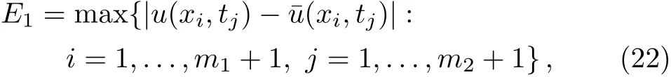
or
where¯u(x,t)is the approximate solution andu(x,t)is the exact solution.
4 The Numerical Examples
In this section,by using the present method,some examples of the Hunter–Saxton equation are solved.To show the effciency and capability of the present method,the obtained results with the corresponding analytical or numerical solutions are compared.
4.1 Example 1
In Eq.(18),it is assumed that:[15]
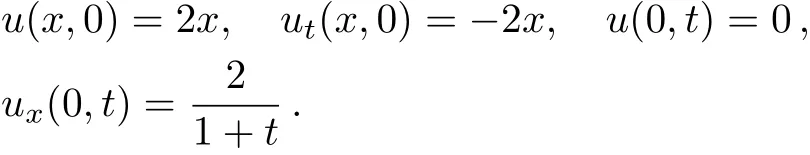
Baxter et al.[14]have proved that the exact solution is as follows:
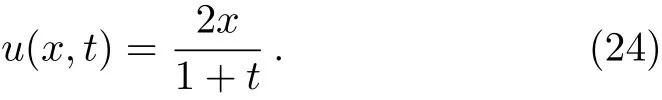
By applying the technique described in the previous section,we have
and the initial guessu0(x,t)=2x−2xt+xt2.It can be seen that they are satisfied in the initial conditions and one of the boundary conditions.
Figure 1 shows the graph of the maximum of the absolute errors for various values ofα.We can see that an appropriate value for the parameter ofαis 1.
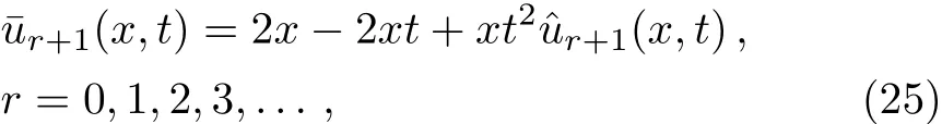
Tables 1–3 show the obtained results of the present method for various values ofx,225 nodes(m1=m2=14),5th iterations,andt=0.1,t=0.01 andt=0.001 respectively,and comparing them with the obtained results by Arbabi et al.[15]using the Haar wavelet quasilinearization approach(HWQA)and the exact solution.It is seen that the obtained results of the present method are more accurate than the previous results.

Fig.1 Graph of the maximum of the absolute errors for various values of α,for example 1.
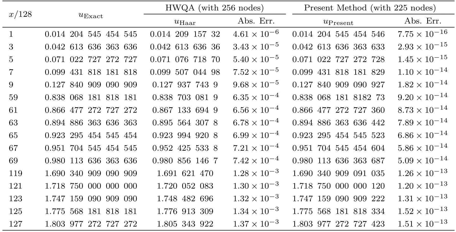
Table 1 Comparing the present method with the obtained results by Ref.[15],for example 1 with t=0.1.
Table 2 Comparing the present method with the obtained results by Ref.[15],for example 1 with t=0.01.
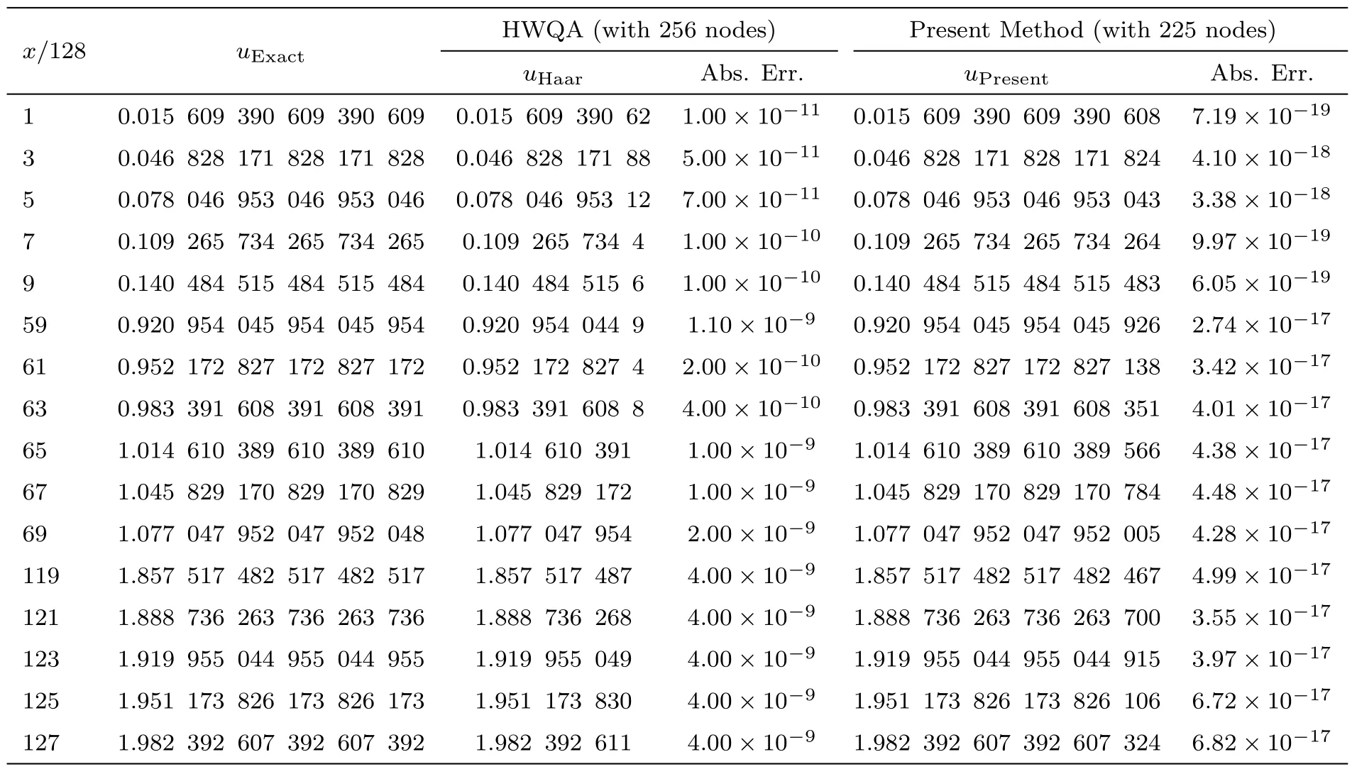
Table 3 Comparing the present method with the obtained results by Ref.[15],for example 1 with t=0.001.

Fig.2 Graphs of the residual error and the absolute error,for example 1.
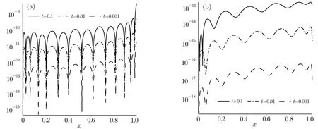
Fig.3 Graphs of the residual errors and the absolute errors,for example 1 with t=0.1,t=0.01 and t=0.001.
Figure 2 shows the graphs of residual error Res5(x,t)of Eq.(20),and the absolute error between the present method and the exact solution(24).
Figure 3 shows the graphs of residual errors Res5(x,t)of Eq.(20),and the absolute errors between the present method and the exact solution(24)fort=0.1,t=0.01,andt=0.001.
4.2 Example 2
In Eq.(18),it is assumed that:[15]

Baxter et al.[14]have proved that the exact solution is as follows:

By applying the technique described in the previous section,we have
and the initial guess

It can be seen that they are satisfied in the initial conditions.
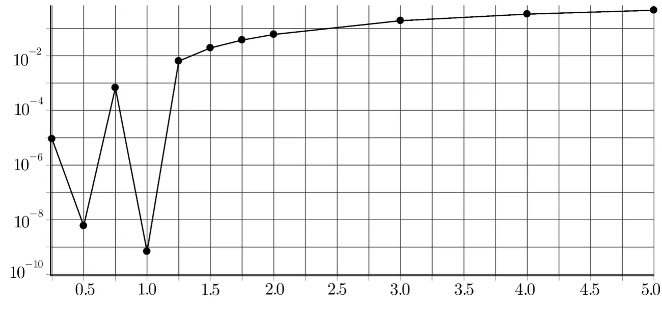
Fig.4 Graph of the maximum of the absolute errors for various values of α,for example 2.
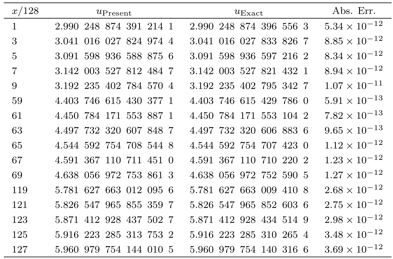
Table 4 Comparing the obtained results by the present method with the exact solution,for example 2 with t=0.1.
Figure 4 shows the graph of the maximum of the absolute errors for various values ofα.We can see that an appropriate value for the parameter ofαis 1.
Tables 4–6 show the obtained results by the present method for various values ofx,225 nodes(m1=m2=14),5th iterations,andt=0.1,t=0.01 andt=0.001 respectively,and comparing them with the exact solution.It is seen that the obtained results by the present method are more accurate.
Figure 5 shows the graphs of residual error Res5(x,t)of Eq.(20),and the absolute error between the present method and the exact solution(26).
Figure 6 shows the graphs of residual errors Res5(x,t)of Eq.(20),and the absolute errors between the present method and the exact solution(26)fort=0.1,t=0.01 andt=0.001.
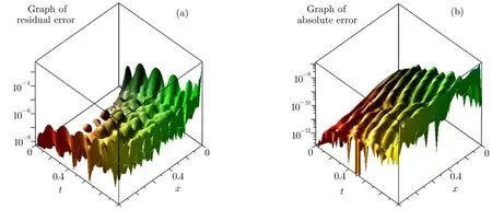
Fig.5 Graphs of the residual error and the absolute error,for example 2.
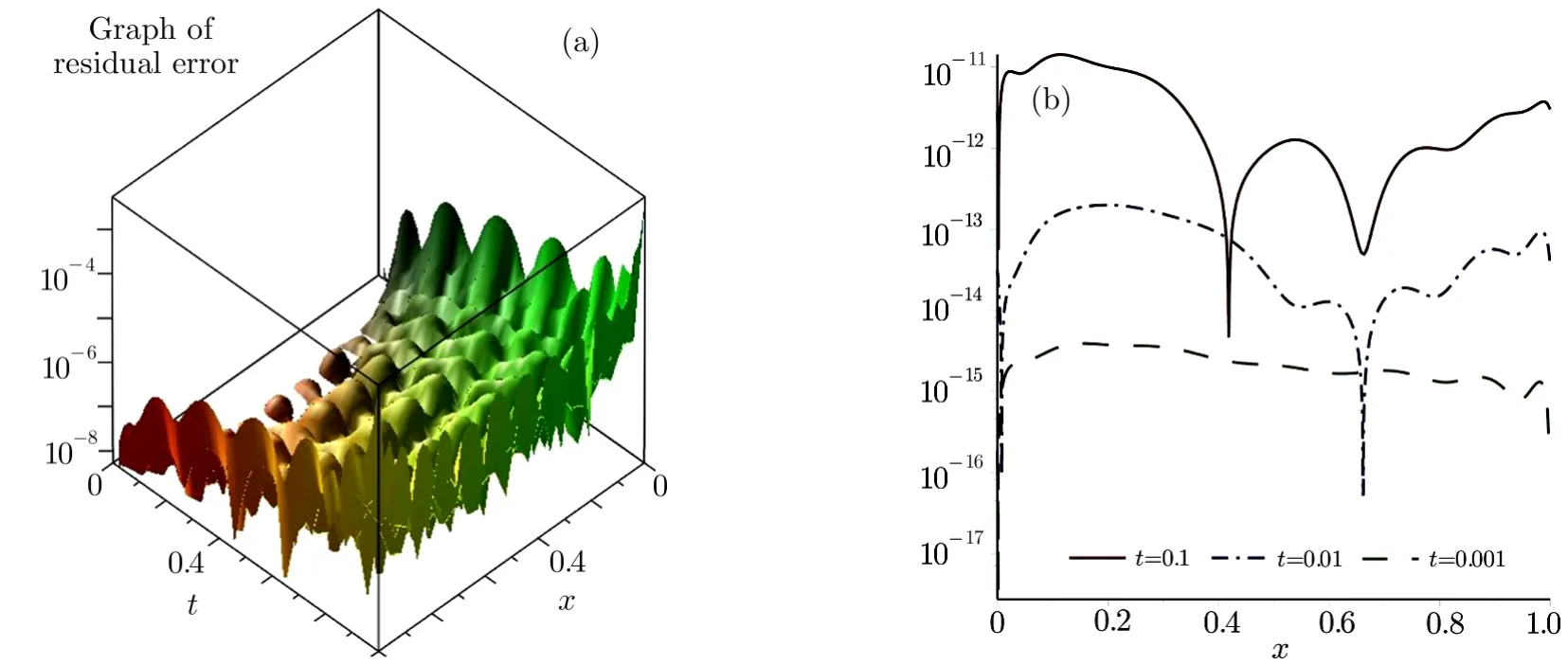
Fig.6 Graphs of the residual errors and the absolute errors,for example 2 with t=0.1,t=0.01,and t=0.001.
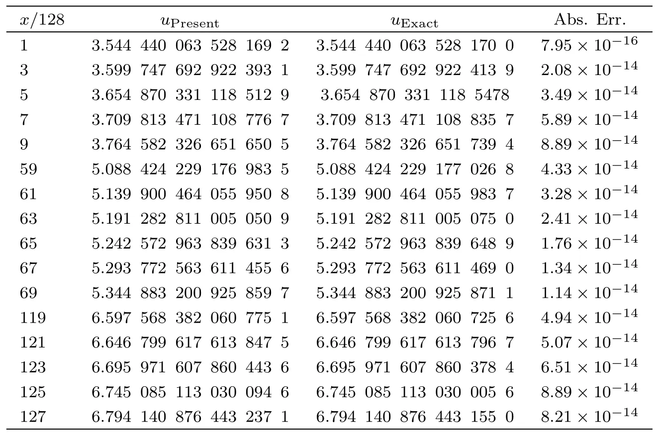
Table 5 Comparing the obtained results by the present method with the exact solution,for example 2 with t=0.01.

Table 6 Comparing the obtained results by the present method with the exact solution,for example 2 with t=0.001.
5 Conclusion
The fundamental goal of the paper has been to construct an approximation to the solution of nonlinear Hunter–Saxton equation.To achieve this goal,a hybrid numerical method based on the quasilinearization method and the bivariate generalized fractional order of the Chebyshev functions(B-GFCF)collocation method is applied.The obtained results of the present method are more accurate than the results that calculated by other methods for fewer collocation points and are in a good agreement with the exact solutions.So it can be concluded that the present method is very convenient for solving other nonlinear partial differential equations.
The authors are very grateful to reviewers and editor for carefully reading the paper and for their comments and suggestions which have improved the paper.
[1]J.K.Hunter and R.Saxton,SIAM J.Appl.Math.51(1991)1498.
[2]R.I.Ivanov,J.Nonlinear Math.Phys.15(2008)1.
[3]R.Camassa and D.D.Holm,Phys.Rev.Lett.71(1993)1661.
[4]P.Olver and P.Rosenau,Phys.Rev.E 53(1996)1900.
[5]R.Beals,D.Sattinger,and J.Szmigielski,Appl.Anal.78(2001)255.
[6]R.Beals,D.Sattinger,and J.Szmigielski,Appl.Anal.78(2000)255.
[7]A.V.Penskoi,Phys.Lett.A 304(2002)157.
[8]Z.Yin,SIAM J.Math.Anal.36(2004)272.
[9]J.Lenells,J.Geom.Phys.57(2007)2049.
[10]Y.Xu and C.W.Shu,J.Comput.Math.28(2010)606.
[11]X.Wei and Z.Yin,J.Nonlinear Math.Phys.18(2011)1.
[12]X.Wei,J.Math.Anal.Appl.391(2012)530.
[13]M.Nadja fikhah and F.Ahangari,Commun.Theor.Phys.59(2013)335.
[14]M.Baxter,R.A.Van Gorder,and K.Vajravelu,Commun.Theor.Phys.63(2015)675.
[15]S.Arbabi,A.Nazari,and M.T.Darvishi,Optik-Int.J.Light Electron Optics 127(2016)5255.
[16]K.Parand and M.Delkhosh,J.Comput.Appl.Math.317(2017)624.
[17]E.B.Baker,Q.Appl.Math.36(1930)630.
[18]A.H.Bhrawy and A.S.Alo fi,Appl.Math.Lett.26(2013)25.
[19]J.A.Rad,S.Kazem,M.Shaban,K.Parand,and A.Yildirim,Math.Method.Appl.Sci.37(2014)329.
[20]E.H.Doha,A.H.Bhrawy,and S.S.Ezz-Eldien,Comput.Math.Appl.62(2011)2364.
[21]A.Saadatmandi and M.Dehghan,Numer.Meth.Part.D.E.26(2010)239.
[22]K.Parand,A.Taghavi,and M.Shahini,Acta Phys.Pol.B 40(2009)1749.
[23]K.Parand,A.R.Rezaei,and A.Taghavi,Math.Method.Appl.Sci.33(2010)2076.
[24]K.Parand and S.Khaleqi,Eur.Phys.J.Plus 131(2016)1.
[25]K.Parand,M.Dehghan,and A.Taghavi,Int.J.Numer.Method.H.20(2010)728.
[26]J.P.Boyd,Chebyshev and Fourier Spectral Methods,Second Edition,Dover Publications,Mineola,New York(2000).
[27]K.Parand and M.Delkhosh,Ricerche Mat.65(2016)307.
[28]S.D.Conte and C.de Boor,Elementary Numerical Analysis:An Algorithmic Approach,McGraw Hill International Book Company,third sub edition,New York(1980).
[29]A.Ralston and P.Rabinowitz,A First Course in Numerical Analysis,Dover Publications,second edition,Mineola,New York(2001).
[30]R.E.Bellman and R.E.Kalaba,Quasilinearization and Nonlinear Boundary-Value Problems,Elsevier Publishing Company,New York(1965).
[31]V.B.Mandelzweig and F.Tabakinb,Comput.Phys.Commun.141(2001)268.
[32]R.Kalaba,J.Math.Mech.8(1959)519.
[33]V.Lakshmikantham and A.S.Vatsala,Generalized Quasilinearization for Nonlinear Problems,Mathematics and its Applications,Vol.440,Kluwer Academic Publishers,Dordrecht(1998).
[34]K.Parand,M.Ghasemi,S.Rezazadeh,A.Peiravi,A.Ghorbanpour,and A.Tavakoli Golpaygani,Appl.Comput.Math.9(2010)95.
[35]R.Krivec and V.B.Mandelzweig,Comput.Phys.Commun.179(2008)865.
[36]E.Z.Liverts and V.B.Mandelzweig,Ann.Phys-New York 324(2009)388.
[37]A.Rezaei,F.Baharifard,and K.Parand,Int.J.Comp.Elect.Auto.Cont.Info.Eng.5(2011)194.
[38]S.S.Motsa,V.M.Magagula,and P.Sibanda,Scient.World J.2014(2014)Article ID 581987.
 Communications in Theoretical Physics2017年5期
- Communications in Theoretical Physics的其它文章
- Elastic Deformation Analysis on MHD Viscous Dissipative Flow of Viscoelastic Fluid:An Exact Approach
- Magnetic Effect Versus Thermal Effect on Quark Matter with a Running Coupling at Finite Densities∗
- Borromean Windows for Three-Particle Systems under Screened Coulomb Interactions∗
- Isotopic Effects on Stereodynamics of the C++H2→ CH++H Reaction∗
- Entropy Generation Analysis in Convective Ferromagnetic Nano Blood Flow Through a Composite Stenosed Arteries with Permeable Wall
- Effects of Interfaces on Dynamics in Micro-Fluidic Devices:Slip-Boundaries’Impact on Rotation Characteristics of Polar Liquid Film Motors∗