
Numerical analyses of ventilated cavitation over a 2-D NACA0015 hydrofoil using two turbulence modeling methods *
2018-05-14 01:43DandanYang杨丹丹AnYu于安BinJi季斌JiajianZhou周加建XianwuLuo罗先武
水动力学研究与进展 B辑 2018年2期
关键词:丹丹
Dan-dan Yang (杨丹丹), An Yu (于安) , Bin Ji (季斌) , Jia-jian Zhou (周加建) ,Xian-wu Luo (罗先武)
1. State Key Laboratory of Hydroscience and Engineering, Tsinghua University, Beijing 100084, China
2. Beijing Key Laboratory of CO2 Utilization and Reduction Technology, Department of Energy and Power Engineering, Tsinghua University, Beijing 100084, China
3. School of Power and Mechanical Engineering, Wuhan University, Wuhan 430072, China
4. Marine Design and Research Institute of China, Shanghai 200011, China
Introduction
The cavitation occurs when the local pressure is close to the vapor pressure of the liquid, with some adverse effects such as noise, vibration and cavitation erosion. The cavitation is known as a complex twophase flow with intractable phenomena in the submerged bodies and the hydraulic machinery[1-4].However, in the marine industry, super cavitation is found to be an effective method to decrease the ship resistance and improve the propulsion performance.For the usual natural cavitation, a very low cavitation number is necessary to obtain the stable super cavity.Hence the ventilated cavitation was proposed and validated as a useful means to create a super cavity[5].The ventilated cavitation was extensively studied by experiments as well as numerical simulations. Kunz et al.[6]presented a theoretical formulation of an implicit and pre-conditioned algorithm to resolve the natural and ventilated cavitation simultaneously. Feng et al.[7]experimentally investigated the dynamics of the“stabilized cavity” for natural and ventilated cavitating flows around an axisymmetric body. They pointed out that the ventilation had little effects on the fluctuation characteristics of the cavity due to the similarity of the frequency spectra of natural and ventilated cavities. Ji et al.[8]proposed a three-component model based on the mass transfer equation to simulate the ventilated cavitation around an underwater vehicle. For the natural cavitation and the ventilated cavitation, it is essential to consider the watervapor interface and the water-air interface appro-priately. Hirt and Nichols[9]proposed a volume of fluid (VOF) method to track the multiphase flow interface by the interface reconstruction technique.Chang et al.[10]developed the level set method to capture the interface with consideration of the surface tension. Yu et al.[11]applied the level set method to the unsteady cavitating flow with air admission around a cylinder vehicle and the numerical results were found to be in fairly good agreement with the experimental data.
To simulate the cavitating flow more precisely,the choice of the turbulence model is very important because the interaction between the cavity interface and the boundary layer is very strong. Many numerical simulations of cavitating flow were carried out based on various turbulence models. The Reynolds average Navier-Stokes (RANS) model such as thek-εmodel was widely used, with less computational resource, but it tends to over-predict the turbulence viscosity. The applications of the large eddy simulation (LES) are to simulate large-scale turbulence eddies by employing the current Navier-Stokes equations. The influence of small scale turbulence eddies on large ones are considered by an approximate model. But the LES requires an adequate computer memory and CPU speed. Direct numerical simulation(DNS) model is the most accurate and expensive method for the whole scale of turbulence. Some hybrid models were proposed to combine the benefit of these methods. Spalart[12]proposed a detached-eddy simulations (DES) model, which is a combination of the RANS and the LES. Girimaji[13]proposed a Partially-averaged Navier-Stokes (PANS) method,which varied from the RANS to the DNS through adjusting two filter-control parameters, i.e., the unresolved-to-total ratios of the kinetic energyfkand the dissipationfε. With a variable value offk,the flow field can enjoy better accuracy than with a constantfk. Huang et al.[14]validated the superiority of the modified PANS (MPANS) model around a backward facing step. Some modifications of the existing models were made for the simulations of cavitating turbulent flows. One modified model is a filter-based model (FBM) originally proposed by Johansen et al.[15]. A length scale limiting function is used on the eddy viscosity to improve the predictive capability of thek-ε turbulence model. Coutier-Delgosha et al.[16]proposed a density corrected model(DCM) to consider the compressibility effects on the turbulence structure, with the RNGk-ε model modified with a density function. Inspired by these studies, Huang et al.[17]proposed a hybrid turbulence model blending the advantages of the FBM and DCM approaches, and the filter-based density corrected model (FBDCM). Yu et al.[18]validated the FBDCM model through an unsteady simulation of the cavitating flow on a NACA66 hydrofoil. A good agreement was shown between the numerical results of the vapor shedding structure and the experiment data.
Recently, the flow structure analysis based on Lagrangian techniques was applied to the unsteady cavitating flow, including the Lagrangian coherent structure (LCS). Tang et al.[19]used the LCS method to investigate the flow structure in multiphase flows.They found that the the LCS can capture the interface of the vortex region. Long et al.[20]utilized the LCS method to investigate the vortex dynamics and the vortex-cavitation interaction in cavitating flows.
In the present work, the ventilated cavitation is tested and simulated around a two-dimensional NACA0015 hydrofoil. The numerical simulations are conducted with the commercial CFD code ANSYS CFX. To study the ventilated cavitation, two advanced turbulence models are applied to obtain better numerical results of the cavitating turbulent flows. The cavity shapes at various ventilated rates are investigated by comparing the numerical calculations with experimental measurements. The LCS method is also used to study the flow mechanism of the unsteady ventilated cavitation.
1. Governing equations
1.1 Level set method
In a homogenous model, it is assumed that a cavitating flow is a kind of multiphase flow, with the fluid being the mixture of three components, the liquid,the vapor and the non-condensable gas (e.g., air, etc.).In the mixture, all components share the same velocity and pressure. The mixture density i.e., ρ and the dynamic viscosity i.e., μ dependent on the local volume fractions of the components, can be defined by using the level set method.
The level set method is a homogeneous Eulerian-Eulerian multiphase model, with the interface between the two different phases represented by a scalar function (the level set function) φ and the Heaviside functionH. The density and the dynamic viscosity for a cavitating flow[10]can be defined as:

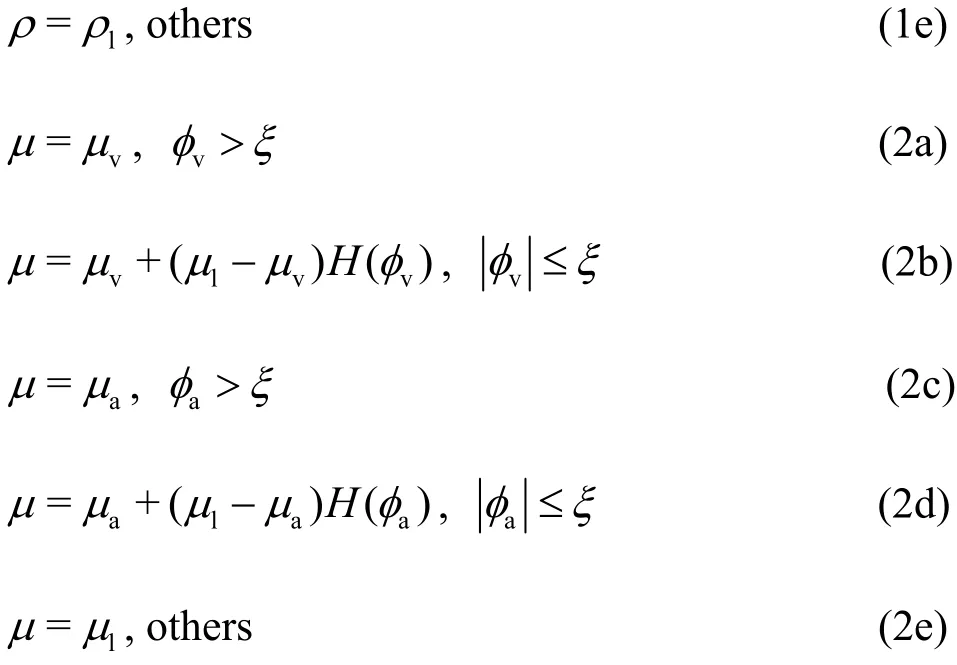
where ξ is a positive small neat parameter, the subscripts l, v and a denote the liquid, the vapor and the air, respectively. The level set functions φ for the water-vapor interface (S1) and the water-air interface (S2) are defined as:

whered1andd2are the shortest distance to the interfacesS1andS2, respectively.
The Heaviside function is defined as:

Thus, based on the level set method, the continuity and momentum conservation equations for a cavitating flow are as follows:


whereuiis the velocity in theidirection,pis the pressure,tμ is the turbulence viscosity given by the turbulence model which would be discussed in detail later.
The last term in the momentum conservation equation is the surface tension force. σis the surface tension coefficient, δ is the Dirac delta function,κis the surface curvature defined by κ=∇⋅, andnis the interface normal vector pointing from the primary to the second fluid defined by. The surface tension force can be described as[10, 11].
1.2 Cavitation model
The cavitation model is a two-phase flow model for predicting the cavitation dynamics based on the Rayleigh-Plesset equation. In the models adopted in the paper, the bubble surface tension and the second order derivative of the bubble radius are neglected.The mass transfer between the liquid and the vapor can be described as

The source terms associated with the vaporization term and the condensation term are as follows:

whereFv=50,Fc=0.01 are the empirical constants for the vaporization and the condensation recommended by Zwart et al.[21],r=5× 10⁻⁴is the nunuccleation site volume fraction andR=1× 10⁻⁶m isbthe typical bubble size in water.
1.3 Turbulence models
Since the cavitating turbulent flows involve the eddy with different scales, the numerical accuracy is closely related with the turbulence modeling method.In this paper, two methods are used for comparison.
1.3.1 FBDCM model
The FBDCM model is built based on the standardk-ε turbulence model, described as:

whereGkdenotes the production term of the turbulence kinetic energy due to the mean velocity gradient.The constants are as follows:C1ε=1.44,C2ε=1.92,σk=1.0 and σε=1.3.
The turbulence viscosity is defined as:

The hybrid function φblends the FBM and DCM turbulence models, which can be described as

whereC1andC2are fixed to 4 and 0.2, respectively[17,18].
1.3.2 MPANS model
The difficulty of the PANS model is to determine the two filter-control parameters, i.e., the unresolvedto-total ratios of the kinetic energyfkand the dissipationfεdefined by

In the turbulence governing equation of the PANS model, the standardk-εturbulence model is treated as the parent RANS model as:

whereGkuis the unresolved production term, and the unresolved kinetic energy σku, the dissipation Prandtl numbers σεuand the value ofare defined by:

The PANS turbulence viscosity is described as

In the MPANS model, the unresolved-to-total ratio of the kinetic energyfkis a variable based on the physical grid (Δ =(Δx*Δy*Δz)1/3) and the local turbulence length scale (l=k1.5/ε)[22], and can be obtained by

2. Numerical implementation
2.1 Computation domain and mesh setup
Figure 1 shows a NACA0015 hydrofoil with a span of 1mm mounted at an attack angle of six degrees in the computation domain. The simulation is conducted using the commercial CFD code ANSYS CFX. The experimental measurements are made in the water tunnel at Beijing Institute of Technology. The chord lengthcof the hydrofoil is 70.0 mm, and there is a ventilated orifice (0.5 mm in width) at the distance of 5.3 mm downstream the leading edge of the hydrofoil.

Fig.1 Computation domain
It should be noted that though in the experiment,a three-dimensional NACA0015 hydrofoil with the span of 70.0 mm is used, in the present paper we mainly focus on the typical cavitation behaviors and a hydrofoil with the span of 1mm is simulated for saving computation resources. This kind of two-dimensional assumption is effective to study the fundamental cavitation shedding dynamics, as is validated by some Refs. [16-18].
After grid independence tests, a structured C-type mesh is generated with 224012 elements in the domain. The mesh near the hydrofoil is refined to meet the requirement of the wall function. The generated mesh around the hydrofoil is illustrated in Fig.2.
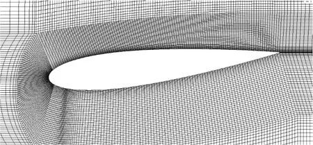
Fig.2 Mesh near the hydrofoil
2.2 Boundary conditions
The boundary conditions are given according to the experimental setup. The Reynolds number is defined byRe=u∞c/ν, and fixed to 5×10⁵, and the cavitation number (p∞-pv)/(0.5ρlu∞2)is 0.65 in the simulation. According to those non-dimensional parameters, the values of the external flow inlet velocity i.e.,u∞and the outlet static pressure i.e.,p∞can be determined. That means that a constant velocity is assigned at the domain inlet, and a static pressure is set at the domain outlet. The front and back surfaces are considered as the symmetry boundaries.The no-slip wall conditions are imposed on the top and the bottom of the water tunnel as well as on the hydrofoil surface. The ventilation rate is characterized by the air flow coefficientCq, which is defined asC=Q/(uc2), whereQis the flow-rate of the airq∞ventilation in the experiment. Three cases with different ventilation rates (Cq=0, 0.001, 0.002) are considered in the simulations.
To capture the unsteady characteristics, the time step of 0.05Trefis chosen in view of an acceptable accuracy and the less computational resource in the simulations. Note thatTrefis the reference period of the cavitation evolution defined byc/u∞.
3. Results and discussions
3.1 Natural cavitation evolution
Five snapshots (10%, 40%, 65%, 90% and 110%in each corresponding cycle) of the transient natural cavitation evolution without air admission predicted by two different turbulence modeling methods are shown in Fig.3. The corresponding experimental results are also presented in the left column for comparison. At the beginning of the evolution as shown in Figs. 3(a1)-3(c1), a thin partial cavity is attached to the leading edge of the hydrofoil. The sheet cavity grows along the surface stably up to the maximum length, as shown in Figs. 3(a2)-3(c2). The cavity is split into two parts as time goes on due to the re-entrant jet, and the front part becomes smaller and eventually disappears,while the rear part is swept to the downstream as shown in Figs. 3(a3)-3(c4). Finally, a new sheet cavity occurs in the next cycle, as shown in Figs. 3(a5)-3(c5).It is noted that the unsteady physical features of the natural cavitation are well captured by both numerical simulations. As a quantitative summary, the results of the cavity shedding frequency obtained by the experiment and the simulations are listed in Table 1. The shedding frequencyfis 22.39 Hz, as recorded by the experimental images. The frequencies of 26.36 Hz and 23.43 Hz are predicted by the FBDCM turbulence model and the MPANS method, respectively. The simulations by both turbulence methods predict larger frequencies than that of the experiment, and the MPANS model yields more accurate numerical results than the FBDCM model. The cavity oscillation frequency discrepancy between the simulation by the MPANS model and the experiment is less 5%, which is acceptable for most engineering applications.

Fig.3 (Color online) The evolution of natural cavitation(Cq=0)

Table 1 Cavity shedding frequency (Cq=0)
3.2 Ventilated cavitation evolution
Figure 4 and Fig.5 illustrate five snapshots (12%,37.5%, 62.5%, 87.5% and 112.5% in each corresponding cycle) of the transient ventilated cavitation using the two different turbulence models at the ventilated rateCq=0.001. In each figure, the left column is the air cavity, and the right column is the vapor cavity. The cavity shedding process of each ventilated cavitation is similar to that of the natural cavitation shown in Fig.3, but the vapor cavity has a smaller volume fraction. The results indicate that the natural cavitation is depressed by the air admission[11].For the ventilated cavitation, there are both the air cavity and the vapor cavity. Since the air is introduced from the hydrofoil surface, the air cavity will push the vapor cavity away from the hydrofoil. Because the pressure outside the air cavity zone may be higher than that near the hydrofoil surface, the vapor cavity would be compressed and shrunk. It is also seen that the air cavity has the same shedding frequency as the vapor cavity, i.e., 27.43 Hz for the FBDCM model and 25.36 Hz for the MPANS model. In both cases,the vapor cavity at the leading edge is inhibited by the injected air at the instant (a4), (b4). At the rear part of the hydrofoil, there is some vapor cavity. The vapor cavity volume obtained by the FBDCM model is much larger than that obtained by the MPANS model,as shown in Figs. 4(b4) , 5(b4).
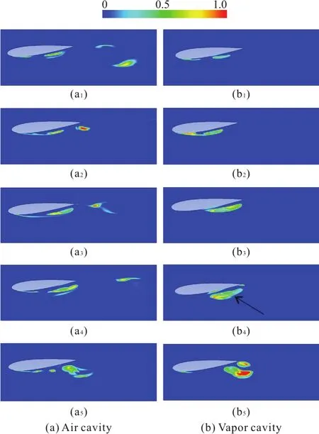
Fig.4 (Color online) The evolution of ventilated cavitation, by FBDCM model (Cq=0.001)

Fig.5 (Color online) The evolution of ventilated cavitation, by MPANS model (Cq=0.001)
Figure 6 illustrates one cavity shedding snapshot at the ventilated rateCq=0.002, which corresponds to the maximum cavity length. At this ventilated rate,the super cavity appears and the periodic shedding of the cavity is not so clear in the experimental observation. With the MPANS model, the predicted super cavity length is in fairly good agreement with the experiment result. However, the super cavity length is over predicted by the FBDCM model.

Fig.6 (Color online) One cavity shedding snapshot (Cq=0.002)
3.3 Cavity volume vibrations
To display the effect of the injected air on the natural cavitation clearly, the vibrations of the air and vapor cavity volumesCvat different ventilated rates are shown in Figs. 7, 8. Before the air injects into the hydrofoil, the average vapor volume is about 2×10⁻⁷m3in the natural cavitation. With the increase of the injected air, the oscillation amplitude of the vapor cavity volume decreases significantly, the average vapor cavity volume is decreased to 0.5×10⁻⁷m3at the ventilated rateCq=0.001. The results indicate that the injected air has an inhibitory effect on the development of the natural vapor cavity. When the ventilated rate increases toCq=0.002, the oscillation amplitude of the vapor cavity volume becomes very small after one to two cycles. The vapor cavity volume is near zero as shown in Figs. 7(b), 8(b),which means that the vapor cavity is completely depressed by the ventilated air. It is also noted that the oscillation amplitude of the vapor cavity predicted by the MPANS model is smaller as compared with that predicted by the FBDCM model, before and after the air ventilation.

Fig.7 Cavity volume variations with different Cq, by FBDCM model

Fig.8 Cavity volume variations with different Cq, by MPANS model
3.4 Drag and lift coefficient distributions
The plots of the drag coefficientCdand the lift coefficientClalong the hydrofoil surface during the simulation at three ventilated rates are shown in Figs.9-12. For convenience, some non-dimensional parametersCd,Cl,t*are defined:Cd=Fx/(0.5ρu∞2A),Cl=Fy/(0.5ρu∞2A),t*=(t-t0)/(t1-t0), whereFx,Fyare the drag and lift forces acting on the hydrofoil,Ais the area for the passing flow, andt0andt1are the start and ending times of the cavitation oscillation period. Table 2 and Table 3 show the drag and lift oscillations predicted by the two turbulence models, respectively. In the tables, ave and amp mean the averaged data and the amplitude of the oscillation, respectively. With the increase of the ventilated rate, the frequency of the cavity oscillation increases. The oscillation frequency becomes very high at the ventilated rateCq=0.002 due to the occurrence of the super cavity. It is noted that with both turbulence methods, similar frequency, aver aged value and amplitude are predicted. Basically, with the FBDCM method, larger frequency and amplitude are estimated than with the MPANS method. With the increase of the ventilated rate, the drag decreases remarkably. At the ventilated rateCq=0.002, the lift drops rapidly.

Fig.9 Drag coefficient versus non-dimensional time t*, by FBDCM model

Fig.10 Drag coefficient versus non-dimensional time t*, by MPANS model

Fig.11 Lift coefficient versus non-dimensional time t*, by FBDCM model

Fig.12 Lift coefficient versus non-dimensional time t*, by MPANS model

Table 2 Drag oscillation

Table 3 Lift oscillation
4. Further considerations
The process of the cavitation evolution is widely displayed through the cavity volume fraction in most researches. In this part, the flow structure in the unsteady cavitating flow is analyzed by different methods for better understanding the cavitation behavior.
4.1 Cavitation-vortex interaction
To better understand the cavitation-vortex interaction, the vorticity transport equation (VTE) is employed as

The first term on the right-hand side (RHS) is called the vortex stretching term, which represents the convection, the stretching and the tilting of the vorticity. In the two-dimensional cavitation flow, the vortex stretching term is zero. The second term on the RHS represents the dilatation due to the volumetric expansion or contraction. The third term on the RHS means the baroclinic torque. The last term on the RHS indicates the viscous diffusion, which has a smaller effect on the vorticity transport compared to other terms in the high Reynolds number flow[23-25]. Hence,only the vortex dilatation term and the baroclinic torque term are considered in this paper.
The contour plots of the vortex dilatation and baroclinic torque terms in one typical cycle predicted by the FBDCM and MPANS models are shown in Figs. 13, 14, corresponding to the snapshots of the cavity volume shown in Figs. 4, 5, respectively. The results indicate that the vortex dilatation term is highly related to the cavity evolution. The vortex dilatation term represents the volumetric expansion or contraction due to the flow compressibility, and is zero in the non-cavitation region. The baroclinic torque term is an important factor in the vorticity field in the regions with high density and pressure gradients, i.e., along the water-vapor interface, the water-air interface and near the cavity closure, but is negligible inside the attached cavity region. It is indicated that the density change cannot be neglected in the case with air admission, especially in the regions where the cavity is lifted off, broken, and transformed into a cloud cavity.
Besides, with the MPANS method, smaller cavity and little weaker vorticity production/depression are predicted as compared with the FBDCM method. However, both methods reveal the close relation between the cavitation development and the vorticity production.

Fig.13 (Color online) Predicted dilatation and baroclinic torque term, by FBDCM model (Cq=0.001)

Fig.14 (Color online) Predicted dilatation and baroclinic torque term, by MPANS model (Cq=0.001)
In Fig.15, the local distribution of the unresolved-to-total ratios of the kinetic energyfkis shown at the ventilated rateCq=0.001. The result shows that the value offkswitches to that outside the cavitation region. In the cavitation region and the wake region, the value offkis relative small,especially near the hydrofoil surface. That means that since in the MPANS method, a dynamicfkis applied, the method is suitable to be used to predict the dynamics for the ventilated cavitation.

Fig.15 (Color online) fk distribution,byMPANSmodel(C q=0.001)
4.2 Lagrangian coherent structure
Further analysis of the flow structure in the ventilated cavitation is made by the Lagrangian coherent structure (LCS) method in the present paper. The detailed formulation can be found in the Ref. [26].The finite-time Lyapunov exponent (FTLE) field is a scalar field, which represents the maximum stretching rate for the fluid particles. The ridge in the FTLE field is named the LCS. Figure 16 shows the FTLE distribution in one typical cycle at the ventilated rateCq=0.001 by the MPANS model. Two main LCSs can be observed at the cavitation region, named the leading edge LCS (LE-LCS) and the trailing edge LCS (TE-LCS), which represent the boundary of the vortex structure. To present the transient process of the vortex dynamics, tracer particles are seeded along the normal of the hydrofoil surface, which are initially located at 0.2cand 0.7cdownstream the leading edge as shown in Fig.17. Different colors represent the locations of tracer particles at different times.Figure 17(a) shows that the tracer particles far away from the hydrofoil surface move downstream following the main flow. However, the movement of the tracer particles near the hydrofoil surface is slower.It means that the tracer particles near the hydrofoil surface are trapped to the LE-LCS due to the attached cavity. In addition, the LE-LCS extends to the trailing edge, which means that the attached cavity may cover the whole pressure side, which can also be verified as shown in Fig.5(a3). Figure 17(b) shows that the tracer particles near the hydrofoil surface firstly move upstream along the suction side and then move downstream. The upstream movement of the tracer particles indicates the existence of the reverse flow,i.e., the re-entrant jet. The tracer particles away from the hydrofoil surface firstly move downstream in order and then separate near the rear part of the hydrofoil. This is because with the shedding of the attached cavity, it gradually develops into a cloud cavity due to the effect of the large vortex structure,which has an impact on the flow field. The tracer particles near the rear part are trapped to the TE-LCS by the shedding cloud cavity, which leads to the separation of the tracer particles in the wake flow.

Fig.16 (Color online) FTLE distribution in one typical cycle,by MPANS model (Cq=0.001)

Fig.17 (Color online) LCSs and tracer particles, by MPANS model (Cq=0.001)
5. Conclusions
In this paper, the experimental investigation and the numerical simulations of the unsteady natural cavitation and the ventilated cavitation are presented.Conclusions can be drawn as follows:
(1) It is verified through comparisons between experimental data and simulated results that with the present numerical methods, the ventilated cavitation with three components (water, vapor and air) can be successfully predicted.
(2) In the ventilated cavitation, the vapor cavity and the air cavity have the same shedding frequency.At the small ventilated rate, the air cavity pushes the vapor cavity away from the hydrofoil surface. As the ventilated rate increases, the vapor cavity is depressed rapidly by the injected air. Further, a suitable air admission can reduce the drag on the hydrofoil surface and achieve a stable operation.
(3) With the FBDCM method, larger oscillation frequency and amplitude are estimated for the cavity,hydrofoil lift and drag coefficients than with the MPANS method, while with the MPANS method,little weaker vorticity production or depression are predicted as compared with the FBDCM method. On the whole, the MPANS method is preferable for engineering applications due to the acceptable accuracy.
(4) The simulation results show the effect of the cavitation on the vortex dynamics. That means that there is a strong cavitation vortex interaction, and the vortex dilatation and baroclinic torque terms are highly dependent on the cavitation evolution.
(5) Two main LCSs are observed at the cavitation region, named the Leading Edge LCS (LE-LCS)and the Trailing Edge LCS (TE-LCS) in the FTLE distribution. The tracer particles initially located at 0.2cand 0.7cdownstream the leading edge reveal the transient process from the attached cavity to the cloud cavity due to the cavity vortex interaction.
Acknowledgements
This work was supported by the Beijing Key Laboratory Development Project (Grant No.Z151100001615006), the Science and Technology on Water Jet Propulsion Laboratory (Grant No.61422230103162223004) and the State Key Laboratory for Hydroscience and Engineering, Tsinghua University (Grant No. sklhse-2017-E-02).
[1] Luo X. W., Ji B., Tsujimoto Y. A review of cavitation in hydraulic machinery [J].Journal of Hydrodynamics, 2016,28(3): 335-358.
[2] Luo X. W., Wei W., Ji B. et al. Comparison of cavitation prediction for a centrifugal pump with or without volute casing [J].Journal of Mechanical Science and Technology,2013, 27(6): 1643-1648.
[3] Peng X. X., Ji B., Cao Y. et al. Combined experimental observation and numerical simulation of the cloud cavitation with U-type flow structures on hydrofoils [J].International Journal of Multiphase Flow, 2016, 79:10-22.
[4] Sedlar M., Ji B., Kratky T. et al. Numerical and experimental investigation of three-dimensional cavitating flow around the straight NACA2412 hydrofoil [J].Ocean Engineering, 2016, 123: 357-382.
[5] Kuklinski R., Castano J., Henoch C. Experimental study of ventilated cavities on dynamic test model [J].CancerResearch, 2001, 73(8 Suppl.): 2400.
[6] Kunz R. F., Boger D. A., Chyczewski T. S. Multi-phase CFD analysis of natural and ventilated cavitation about submerged bodies [C].3rd ASME/JSME Joint Fluids Engineering Conference, San Francisco, California, USA,1999.
[7] Feng X. M., Lu C. J., Hu T. Q. The fluctuation characteristics of natural and ventilated cavities on an axisymmetric body [J].Journal of Hydrodynamics, 2005, 17(1):87-91.
[8] Ji B., Luo X. W., Peng X. X. et al. Numerical investigation of the ventilated cavitating flow around an underwater vehicle based on a three-component cavitation model [J].Journal of Hydrodynamics, 2010, 22(6):753-759.
[9] Hirt C. W., Nichols B. D. Volume of fluid (VOF) method for the dynamics of free boundaries [J].Journal of Computational Physics, 1981, 39(1): 201-225.
[10] Changa Y. C., Houa T. Y., Merriman B. et al. A level set formulation of Eulerian interface capturing methods for incompressible fluid flows [J].Journal of Computational Physics, 1996, 124(2): 449-464.
[11] Yu A., Luo X. W., Ji B. Analysis of ventilated cavitation around a cylinder vehicle with nature cavitation using a new simulation method [J].Science Bulletin, 2015, 60(21):1833-1839.
[12] Spalart P. Trends in turbulence treatments [C].Fluids 2000 Conference and Exhibit. Denver, USA, 2000.
[13] Girimaji S. S. Partially-averaged Navier-Stokes model for turbulence: A Reynolds-averaged Navier-Stokes to direct numerical simulation bridging method [J].Journal of Applied Mechanics, 2006, 73(3): 413-421.
[14] Huang R., Luo X., Ji B. et al. Turbulent flows over a backward facing step simulated using a modified partiallyaveraged Navier-Stokes model [J].Journal of Fluids Engineering, 2017, 139(4): 044501.
[15] Johansen S. T., Wu J., Wei S. Filter-based unsteady RANS computations [J].International Journal of Heat and Fluid Flow, 2004, 25(1): 10-21.
[16] Coutier-Delgosha O., Patella R. F., Reboud J. L. Evaluation of the turbulence model influence on the numerical simulations of unsteady cavitation [J].Journal of Fluids Engineering, 2001, 125(1): 38-45.
[17] Huang B., Chen G. H., Zhao J. et al. Filter-based density correction model for turbulent cavitating flows [C].26th IAHR Symposium on Hydraulic Machinery and Systems,Beijing, China, 2012.
[18] Yu A., Ji B., Huang R. F. et al. Cavitation shedding dynamics around a hydrofoil simulated using a filter-based density corrected model [J].Science China Technological Sciences, 2015, 58(5): 864-869.
[19] Tang J. N., Tseng C. C., Wang N. F. Lagrangian-based investigation of multiphase flows by finite-time Lyapunov exponents [J].Acta Mechanica Sinica, 2012, 28(3):612-624.
[20] Long X., Cheng H., Ji B. et al. Large eddy simulation and Euler-Lagrangian coupling investigation of the transient cavitating turbulent flow around a twisted hydrofoil [J].International Journal of Multiphase Flow, 2018, 100:41-56.
[21] Zwart P., Gerber A., Belamri T. A two-phase flow model for predicting cavitation dynamics [C].Fifth International Conference on Multiphase Flow, Yokohama, Japan, 2004.
[22] Girimaji S., Abdolhamid K. Partially-averaged Navier Stokes model for turbulence: Implementation and validation [C].43rd AIAA Aerospace Sciences Meeting andExhibit-Meeting Papers, Reno, Nevada, USA, 2005.
[23] Ji B., Long Y., Long X. P. et al. Large eddy simulation of turbulent attached cavitating flow with special emphasis on large scale structures of the hydrofoil wake and turbulence-cavitation interactions [J].Journal of Hydrodynamics, 2017, 29(1): 27-39.
[24] Huang B., Zhao Y. Wang G. Large eddy simulation of turbulent vortex-cavitation interactions in transient sheet/cloud cavitating flows [J].Computers and Fluids, 2014,92(3): 113-124.
[25] Ji B., Luo X., Arndt R. E. A. et al. Large eddy simulation and theoretical investigations of the transient cavitating vortical flow structure around a NACA66 hydrofoil [J].International Journal of Multiphase Flow, 2015, 68:121-134.
[26] Shadden S. C., Lekien F., Marsden J. E. Definition and properties of Lagrangian coherent structures from finitetime Lyapunov exponents in two-dimensional aperiodic flows [J].Physica D Nonlinear Phenomena, 2005,212(3-4): 271-304.
猜你喜欢
数学小灵通(1-2年级)(2022年5期)2022-06-01
中学生学习报(2022年3期)2022-03-21
数学小灵通(1-2年级)(2022年3期)2022-03-17
数学小灵通(1-2年级)(2022年3期)2022-03-17
人文天下(2021年10期)2022-01-26
大众文艺(2021年14期)2021-08-15
阅读(快乐英语中年级)(2020年11期)2020-12-28
青年生活(2020年5期)2020-03-27
海峡姐妹(2020年1期)2020-03-03
阅读(快乐英语中年级)(2019年2期)2019-09-10
- 水动力学研究与进展 B辑的其它文章
- Revisit submergence of ice blocks in front of ice cover-an experimental study *
- Analytical approach to entropy generation and heat transfer in CNT-nanofluid dynamics through a ciliated porous medium *
- Couple stress fluid flow in a rotating channel with peristalsis *
- 2-D eddy resolving simulations of flow past a circular array of cylindrical plant stems *
- Energy dissipation of slot-type flip buckets *
- Some notes on numerical simulation and error analyses of the attached turbulent cavitating flow by LES *