
On the Generalized Heisenberg Supermagnetic Model∗
2018-06-11 12:21ZhaoWenYan颜昭雯XiaoJingZhang张晓晶RongHan韩荣andChuanZhongLi李传忠
Zhao-Wen Yan(颜昭雯),Xiao-Jing Zhang(张晓晶),Rong Han(韩荣),and Chuan-Zhong Li(李传忠)
1School of Mathematical Sciences,Inner Mongolia University,Hohhot 010021,China
2Department of Mathematics,Ningbo University,Ningbo 315211,China
1 Introduction
The nonlinear σ-models and their supersymmetric extensions have received a lot of attention[1]due to the widely application in gravity theory,[2]the theory of strings[3]and superstrings.[4]The simplest version of the nonlinear σ-model is the Heisenberg ferromagnet(HF)model,which reads as[5]
where S is the spin vector and satisfies the constraint S2=1.It is well known that the HF model is gauge equivalent and geometrical equivalent to the nonlinear Schrödinger equation(NLSE).[6−7]Growing interest has been focused on the extension of the HF model.[8−12]Kundu[13]constructed a deformed HF model and presented that it is gauge equivalent to the mixed derivative NLSE(MDNLSE),which plays an important role in explaining nonlinear propagation of Alfven wave[14]and ultrashot light pulse propagation in the optical fi ber.[15]Recently,Levin et al.[16]investigated the relation between the deformed HF model and the quantum 11-vertex R-matrix.By constructing the classical integrable tops,they establish more complicated integrable systems in terms of the quantum R-matrices.
More motivations come from supersymmetric integrable systems involving the supersymmetric extension of the important integrable systems.[17−22]The Heisenberg supermagnet(HS)model is the super extension of the HF model.It has attracted considerable interest in the study of the HS model and its corresponding gauge equivalent counterpart.[23]It should be noted that the HS model has close relation with the strong electron correlated Hubbard model.Ghose Choudhury and Roy Chowdhury[24]analyzed the nonlocal conservation laws and the corresponding supercharges in the HS model.Lately,the generalization of the integrable HS models attracts a lot of interest.The structure and integrability properties of the generalized HS models have been well discussed.[25−29]The purpose of this paper is to construct an extension of the HS model and to investigate their integrability.
The organization of this paper is as follows.In Sec.2,we recall the HS model and its integrable properties.Section 3 is dedicated to constructing the super generalized HS model and to deriving the Lax representation with two constraints.Using the gauge transformation,we study their gauge equivalent counterparts.In Sec.4,we end this paper with a summary and discussion.
2 HS Model
For later convenience,we shall recall the definitions of the HS model in this section.For a more detailed description we refer the reader to Ref.[23].
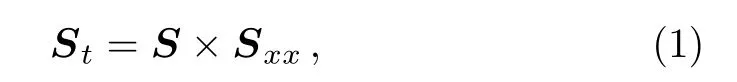
Being the superextensions of the HF model,the HS model reads as
where S is the superspin variable and can be represented
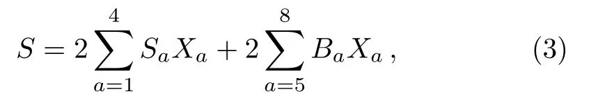
whereS1,...,S4arethebosonic componentsand B5,...,B8are the fermionic ones,X1,...,X4are bosonic generators and X5,...,X8are fermionic generators of the superalgebra uspl(2/1).They can be written as
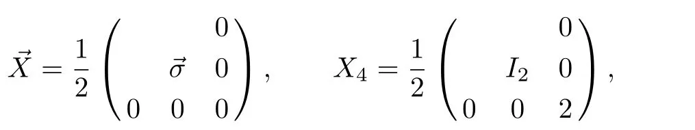
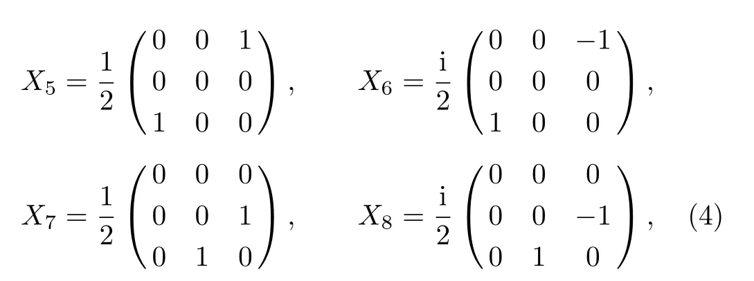
where= σ1,σ2,σ3are Pauli matrices and I2is an identity matrix.
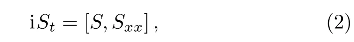
The gauge equivalence is an important concept in the integrable systems.Such interconnections allow us not only to understanding the structure and properties of nonlinear systems already known,but also to conclude about the properties of a system knowing the corresponding properties of its gauge-equivalent counterpart.One can also consider the gauge equivalence of the supersymmetric integrable systems. Under the two constraints(I)S2=S for S∈USPL(2/1)/S(L(1/1)×U(1))and(II)S2=3S−2I for S∈USPL(2/1)/S(U(2)×U(1))Makhankov and Pashaev[23]showed the HS model(2)is gauge equivalent to supersymmetric NLSE and Grassman odd NLSE,respectively
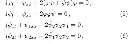
where φ(x,t)is a bosonic filed and ψ, ψ1, ψ2are the fermionic fileds.
3 Generalized Heisenberg Supermagnetic Model
Considering the deformation of the HS model under the constraint I.S2=S,one easily gets SStS=0 and S[S,Sxx]S=0.Now we suppose the generalized HS model as follows

where f is the function of x and t,p and q need to be determined later.For the constraint I,it is not difficult to check S[S,Sx]S=0,SSxS=0.We now take
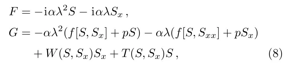
where λ is the spectral parameter.
The zero-curvature condition equation
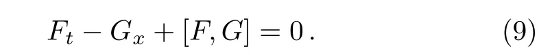
Substituting Eq.(8)into Eq.(9),we obtain
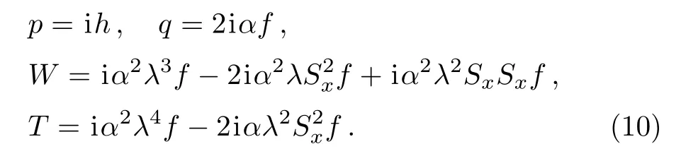
Then we rewrite Eq.(7)as the expression

Now we will mainly be concerned with Eq.(11)in the frame work of the gauge equivalent.Proceeding the similar procedure as,[23]we suppose

where g(x,t)∈USPL(2/1).
Under the constraint I and II,we take Σ=diag(0,1,1)and Σ=diag(1,1,2),respectively.Then we introduce the currents
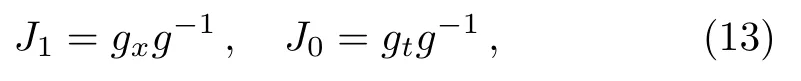
satisfying the condition

Let us decompose the super algebra uspl(2/1)into two orthogonal parts
here[L(i),L(j)}⊂L(i+j)mod(2).L(0)is an algebra constructed by means of the generators of the stationary subgroup H.The stationary subgroup H is S(L(1/1)×U(1))and S(U(2)×U(1))for constraint I and II,respectively.
Taking
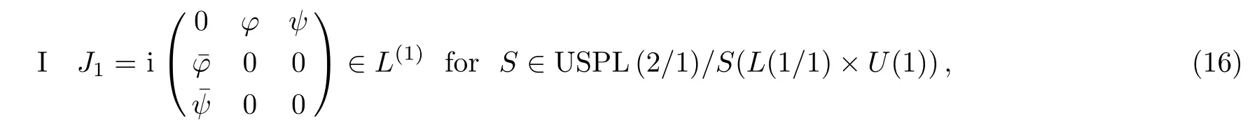
where φ(x,t)and ψ(x,t)are the bosonic and fermionic field,respectively.
Using Eqs.(12),(13),and(16),we obtain

Substituting Eq.(17)into Eq.(11),we have

Equation(18)leads totakes the form
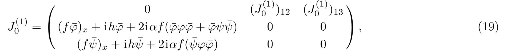
where
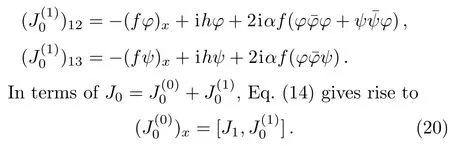
Substituting Eqs.(16)and(19)into Eq.(20)and integrating Eq.(20),we have
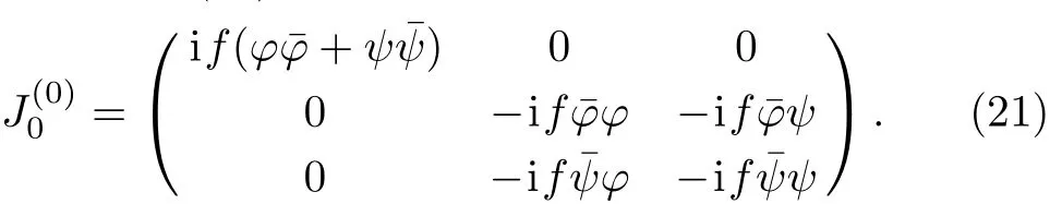
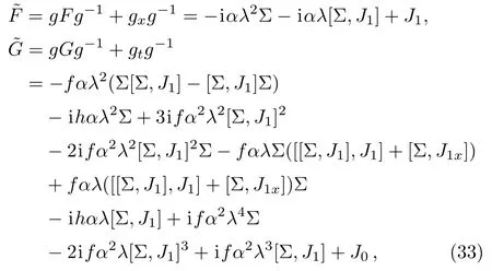
By mean of Eqs.(20),(21),and J0=+,we obtain J0.In terms of the gauge transformation,F and G in Eq.(8)becomeˆF andˆG,respectively,
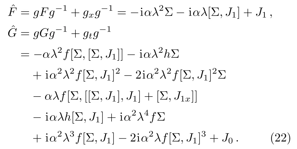
Substituting Σ=diag(0,1,1),Eqs.(20)and(21)into Eq.(22),we have
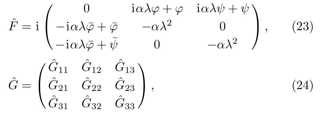
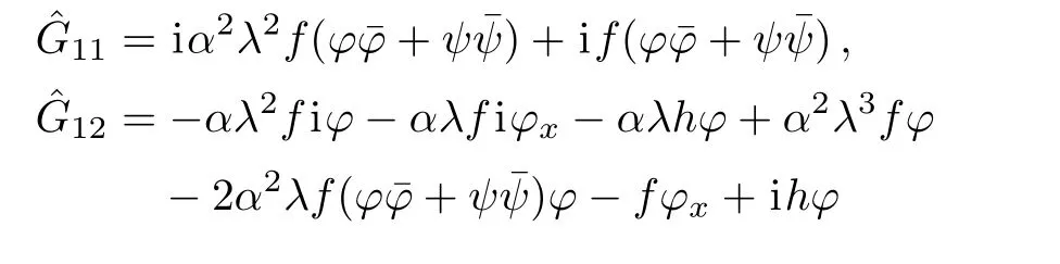
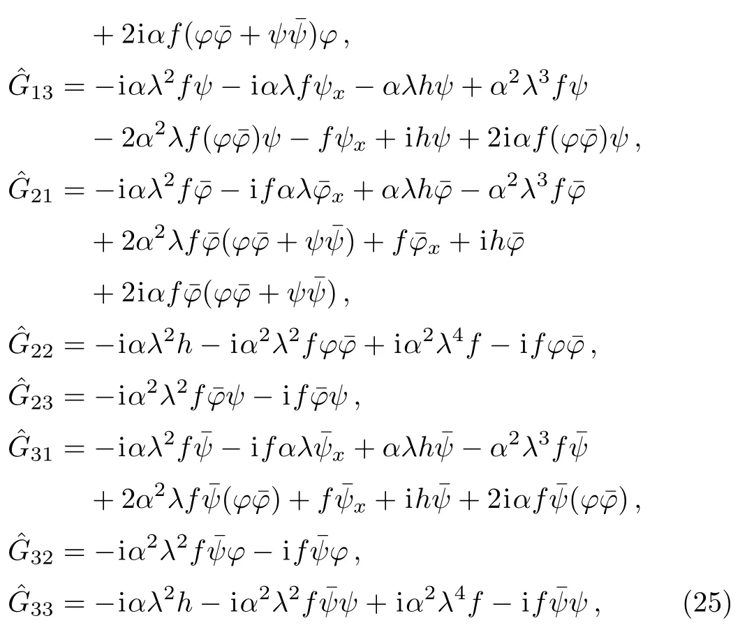
where
where the spectral parameter λ satis fies λt= λx=0.
The zero-curvature condition equation ofˆF andˆG gives the super generalized MDNLSE
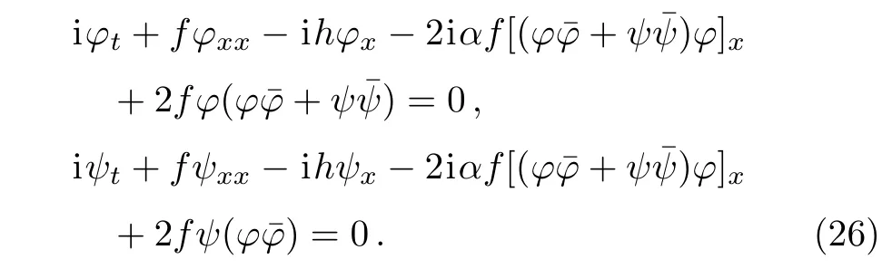
Under the reduction f=1,h=0,Eq.(26)reduces to the super MDNLSE.[25]In the bosonic limit and f=1,h=0,Eq.(26)leads to the MDNLSE.[13]
Let us take account of the generalized HS model(11)with the constraint II.It should be noted that the expression of the corresponding integrable extension is also Eq.(11).For this case,the corresponding F and G are
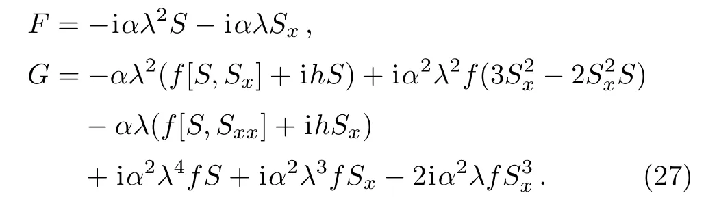
As was done in the constraint I,we consider
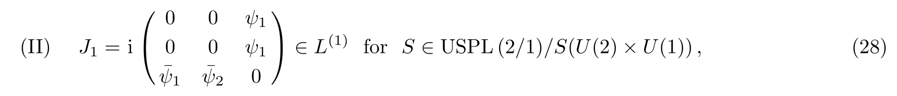
where ψ1(x,t),ψ2(x,t)are the fermionic fields.Using the similar methods as shown before,we easily carry out
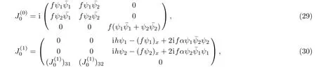
where

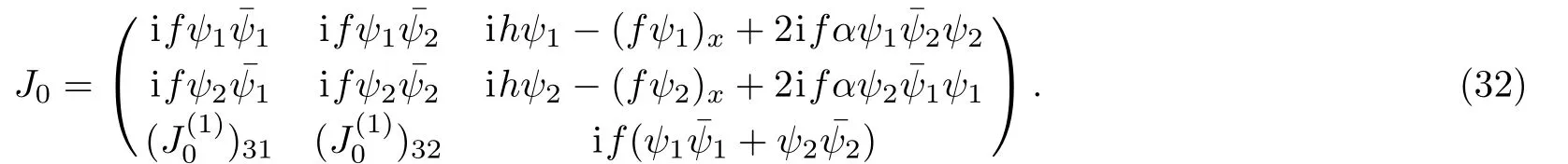
Combining Eqs.(29)and(30),we have
Based on the gauge transformation,F and G turn toandrespectively,
where Σ=diag(1,1,2).
By virtue of Eqs.(28)and(32),we rewrite Eq.(33)as follows
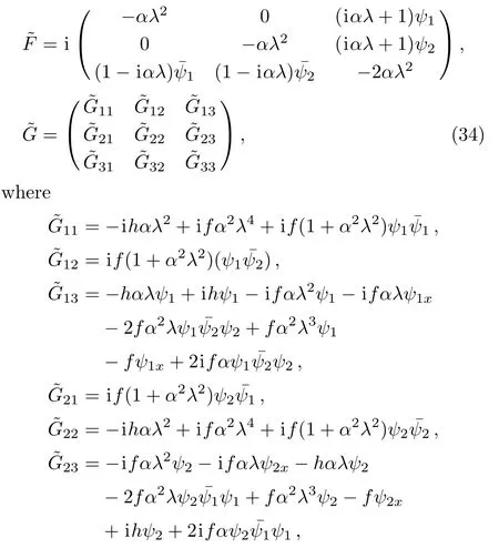

where the spectral parameter λ satis fies λt= λx=0.
From the zero-curvature condition equation ofandwe obtain the generalized fermionic MDNLSE
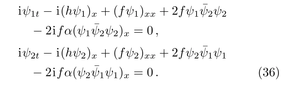
Introducing the reduction f=1 and h=0,Eq.(36)leads to the fermionic MDNLSE.[25]
4 Summary and Discussion
We construct the generalization of the HS model with two different constraints.The Lax pairs associated with the generalized models have been deduced.By means of the gauge equivalence,the related super MDNLSEs are derived,which can be regarded as the generalized super MDNLSEs.There has been a considerable interest in the study of the strong electron correlated Hubbard model due to its important applications in physics.Therefore,as to the applications of the integrable generalized HS models presented in this paper,their applications in physics still deserve further study.
Acknowledgments
The authors thank the valuable suggestions of the referees.
[1]R.Geroch,J.Math.Phys.12(1971)918.
[2]F.Ernst,Phys.Rev.167(1968)1175.
[3]A.A.Zheltukhin,Theor.Math.Fiz.52(1982)73.
[4]D.Nemerschansky and S.Yankielowicz,Phys.Rev.Lett.54(1985)620.
[5]V.E.Zakharov and L.A.Takhtadzhyan,Theor.Math.Phys.38(1979)17.
[6]M.Lakshmanan and S.Ganesan,J.Phys.Soc.Jpn.52(1983)4031.
[7]M.Lakshmanan and S.Ganesan,Physica A 132(1985)117.
[8]A.V.Mikhailov and A.B.Shabat,Phys.Lett.A 116(1986)191.
[9]K.Porsezian,K.M.Tamizhmani,and M.Lakshmanan,Phys.Lett.A 124(1987)159.
[10]M.Lakshmanan,K.Porsezian,and M.Daniel,Phys.Lett.A 133(1988)483.
[11]W.Z.Zhao,Y.Q.Bai,and K.Wu,Phys.Lett.A 352(2006)64.
[12]J.F.Guo,S.K.Wang,K.Wu,et al.,J.Math.Phys.50(2009)113502.
[13]A.Kundu,J.Math.Phys.25(1984)3433.
[14]D.J.Kaup and A.C.Newell,J.Math.Phys.19(1978)798.
[15]A.A.Zabolotskii,Phys.Lett.A 124(1987)500.
[16]A.Levin,M.Olshanetsky,and A.Zotov,Nucl.Phys.B 887(2014)400.
[17]P.Di Vecchia and S.Ferrara,Nucl.Phys.B 130(1977)93.
[18]M.Chaichian and P.Kulish,Phys.Lett.B 78(1978)413.
[19]Yu.Manin and A.Radul,Commun.Math.Phys.98(1985)65.
[20]P.Mathieu,J.Math.Phys.29(1988)2499.
[21]D.Sarma,Nucl.Phys.B 681(2004)351.
[22]Z.Popowicz,Phys.Lett.A 354(2006)110.
[23]V.G.Makhankov and O.K.Pashaev,J.Math.Phys.33(1992)2923.
[24]A.Ghose Choudhury and A.Roy Chowdhury,Int.J.Theor.Phys.33(1994)2031.
[25]Z.W.Yan,M.L.Li,K.Wu,and W.Z.Zhao,Commun.Theor.Phys.53(2010)21.
[26]Z.W.Yan,M.R.Chen,K.Wu,and W.Z.Zhao,J.Phys.Soc.Jpn.81(2012)094006.
[27]Z.W.Yan,M.L.Li,K.Wu,and W.Z.Zhao,J.Math.Phys.54(2013)033506.
[28]Z.W.Yan and Gegenhasi,J.Nonlinear Math.Phys.23(2016)335.
[29]Z.W.Yan,M.N.Zhang,D.Y.Ren,et al.,Z.Naturforsch.A 72(2017)331.
 Communications in Theoretical Physics2018年5期
- Communications in Theoretical Physics的其它文章
- New Double-Periodic Soliton Solutions for the(2+1)-Dimensional Breaking Soliton Equation∗
- Seiberg-Witten/Whitham Equations and Instanton Corrections in N=2 Supersymmetric Yang-Mills Theory∗
- Modeling Chemically Reactive Flow of Sutterby Nano fluid by a Rotating Disk in Presence of Heat Generation/Absorption
- Study on the Reduced Traffic Congestion Method Based on Dynamic Guidance Information∗
- Electrical Properties of an m×n Hammock Network∗
- Searches for Dark Matter via Mono-W Production in Inert Doublet Model at the LHC∗