Localized Excitations of a Generalised Jimbo-Miwa Equation∗

Qian Xia(夏骞)and Sen-Yue Lou(楼森岳),2,†

1Physics Department and Ningbo Collaborative Innovation Center of Nonlinear Hazard System of Ocean and Atmosphere,Ningbo University,Ningbo 315211,China

2Shanghai Key Laboratory of Trustworthy Computing,East China Normal University,Shanghai 200062,China

1 Introduction

Recently,exact algebraic related localized solutions including rogue waves,lumps and interactions among algebraic solitons and exponentially localized solitons become one of the hot topics in nonlinear science and many related applied physical fields such as the nonlinear optics,[1−2]plasmas,[3−4]atmosphere,[5−6]Bose-Einstein condensations(BECs)[7]and financial problems.[8]

To find exact solutions of nonlinear systems,the Hirota’s bilinear method is one of the simplest and effective methods.[9−11]However,there are many physically important systems can not be changed to appropriate bilinear systems by only using Hirota’s bilinear operators.It is interesting to extend Hirota’s bilinear operators such that more physically important systems can be cast to suitable bilinear forms with extended bilinear operators.

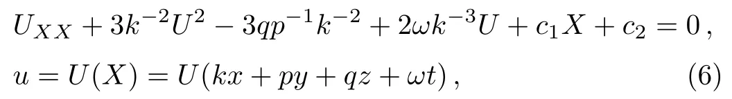
The Jimbo-Miwa(JM)equation[12]

is one of the well known(3+1)-dimensional conditional integrable nonlinear systems to study(3+1)-dimensional nonlinear dynamics.The JM model possesses a bilinear form,

with the relation

where the bilinear operators Dxi,xi=x,y,z,t are defined by

The JM model is also an important member of the so-called Kadomtsev-Petviashvilli(KP)hierarchy.In this short paper,we extend the Hirota’s operator to a more general form.Using the generalized bilinear operators,the usual JM equation can be extended to a new general form with some arbitrary constants.Using the similar solution ansatz method for many integrable and nonintegrable systems like the(extended)KP equation[13]and the extended KdV equations,[14]one can find some novel types of localized excitations in(3+1)dimensions.For instance,under some special model parameter conditions for the generalized JM equation,one can readily find the lump-type line solitons,lumpoff-type half-line solitons and segment solitons.

2 Generalized Bilinear Operators and Generalized Jimbo-Miwa Equation

Various interesting properties of the JM model have been studied by many scientists.For instance,Though the JM equation(1)itself is not integrable(say,not Painlevé integrable),it is really(Painlev’e)integrable under the KP constraint,i.e.,under the KP condition[15]

By using the Lie point symmetry reduction method,one can find many(2+1)-dimensional and(1+1)-dimensional completely integrable systems from the JM equation(1)such as the KP equation,the asymmetric Nizhnik-Novikov-Veselov equation and so on.[16]The existence of the bilinear form(4)implies that the existence of two plane soliton solutions.[17]The traveling wave solutions of the JM equation(1),general solutions of,

have been studied by many authors,say in Ref.[18].Variable separation solutions of the JM equation(1)have been studied by Tang and Liang.[19]Extended Gram-type determinant method and direct ansatz via Maple are used to find rational solutions(lump-type solutions)of the JM equation.[20−21]For a special(2+1)-dimensional reduced JM equation(1),Zhang and Chen have found the lump solution and rogue wave solutions.[22]

To find more general interesting exact solutions of the(3+1)-dimensional JM equation(1),we extend the JM system to a more general form by extending the bilinear operators to more general froms.It is interesting that the bilinear form(2)of the JM equation can be equivalently rewritten as

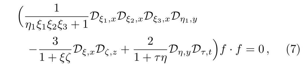
where the generalized bilinear operators Dα,xi,xi=x,y,z,t are defined by

with arbitrary constant α and five constant conditions

among eight parameters ξ,ξ1,ξ2,ξ3,η,η1,ζ,and τ.It is clear that the usual bilinear operator Dxiis just the special case of the generalized bilinear operator Dα,xifor α=−1.

Now,by re-scaling the space-time variables,it is reasonable to extend the bilinear JM equation(7)to the form

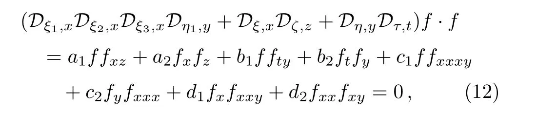
with eight arbitrary constants{ξ,ξ1,ξ2,ξ3,η,η1,ζ,τ} ≡ Ξ without conditions(9),(10),and(11),where

The usual bilinear JM system is equivalent to Eq.(7)(i.e.,Eq.(4))if the conditions(9),(10),and(11)are satisfied.

3 Lump-Type Line Solitons of the Generalized JM Equation

In Ref.[13],it is pointed out that various bilinear systems possess the following types of polynomial solutions

which are related to the lump or lump-type of solutions.

It is interesting that what is the existence condition of Eq.(15)for the generalized bilinear JM equation(12).Substituting Eq.(15)into Eq.(12)and vanishing the coefficients of the different powers of{x,y,z,t},we have the following 15 algebraic equations for 5m+1 solution parameters{ki,pi,qi,ωi,αi}and 8 model parameters{a1,a2,b1,b2,c1,c2,d1,d2},

where the dot product between two m component vectors is defined as usualAfter some tedious but simple direct calculations with helps of the Maple software,the fifteen equations(16)–(30)can be simply solved by the following solution parameter conditions

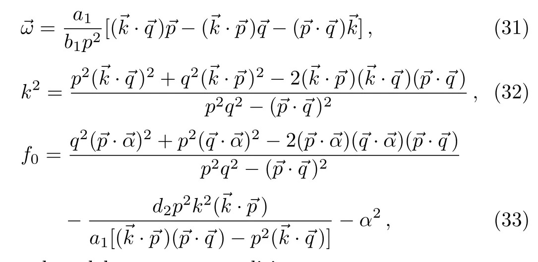
and model parameter conditions

In fact,the condition(34)is just the condition(9)because of Eq.(13).

To verify or prove the correctness of Eq.(31),one can define the vector,

Using the relations(31)and(32),it is straightforward to prove the following identities

The identity(36)for=implies

Using the identities(36)and(37),to verify Eqs.(16)and(30)becomes an easy work.

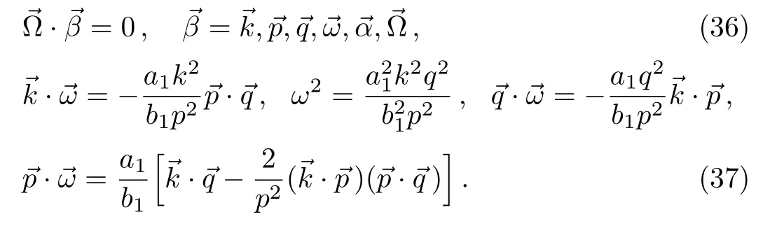
Because of the condition(32),one can prove that the field u related to Eqs.(3)and(15)is only an algebraic line lump-type of soliton solution for all m2.Figure 1 shows a special evolution of the line lump-type solution(3)and(15)with n=4 and the parameter selections

From Fig.1,one can see that for any(2+1)-dimensional reduction,say,

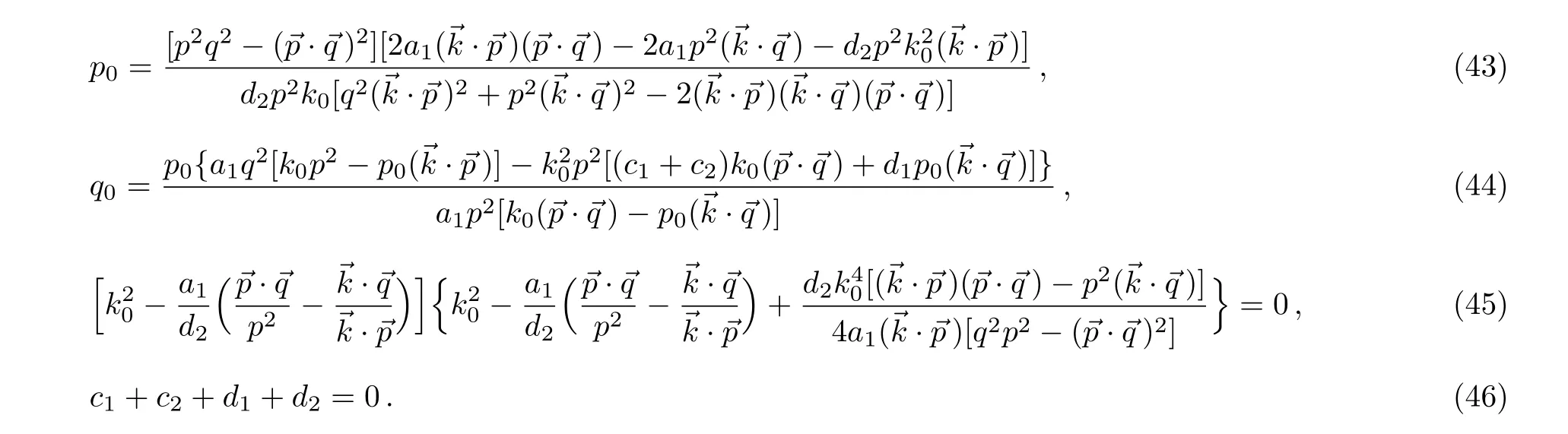
the lump-type line soliton becomes a real lump solution,which is localized in all direction and exists in all time,−∞

Fig.1 The evolution plot of the lump-type of line soliton solution(3)with Eq.(15)for n=4,u=17.4 and the parameter selections(39)at times t=−1,t=0 and t=1 respectively.

4 Lumpo ff-Type Half-Line Soliton Solution Interacted with Exponentially Localized Plane Soliton

From Ref.[13],we know that for various nonlinear systems no matter it is integrable or not there are some kinds of interaction solutions among lump(type)of solitons and exponentially localized solitons in the form

where ξ is completely same as in Eq.(15)including the parameter selections(31),(32),and(33)with arbitrary constant a.

Substituting Eq.(41)into Eq.(12),vanishing coefficients of the different powers of{x,y,z,t}and the exponential factor ek0x+p0y+q0z+ω0tand using the relations(31),(32),(33),and(34)yield the following further conditions

The model parameter conditions(34)and(46)present the existence conditions of the solution(41)for the generalized bilinear JM equation(12).

The solution parameter condition(45)indicates that there exist six possible solutions

for the constant k0,which is completely determined by the inner products of the vectorsWhence k0is fixed from Eq.(47)or Eq.(48),other three constants p0,q0and ω0are also fixed via Eqs.(42),(43),and(44),respectively.

From Eqs.(42)–(45),we know that the exponential part is induced by the algebraic lump-type part.If there is no algebraic part,then there is no exponential part.From Eq.(41),we know that if there is no exponential part(a=0),the solution is only an algebraic lumptype line soliton as mentioned in the last section.When X0≡k0x+p0y+q0z+ωt−→+∞,the algebraic part can be neglected.In other words,the algebraic lump-type of line soliton exists only in half space-time for X0<0.

Figure 2 shows the lumpoff-type half line soliton structure for the field u given by Eq.(3)with Eq.(41)under the same parameter selections as those of Fig.1 except for

at time t=0.

From Fig.2(a),we can find that for the large value of u≤umaxonly the lumpoffpart(half line soliton extended to the area X0≤0)is existed.From Fig.2(b),one can observe both the lump-type half line soliton and the exponentially localized plane soliton for the small value of u,which is less than the maximum of the plane soliton.

From Fig.2,one can see that for any(2+1)-dimensional reduction,say,Eq.(40)the lumpoff-type line soliton becomes a real lumpoff solution,which is localized in all direction and exists only before or after a special time,i.e.,t≤t0or t≥t0.[13]

Fig.2 The plot of the lumpoff-type of half line soliton solution(3)with Eq.(15)for n=4 and the same parameter selections(39)except for Eq.(49),where the value of the field u is fixed as(a)u=10 at time t=−0.5 and(b)u=2.1228 at time t=2,respectively.

5 Algebraic Segment Soliton Interacted with Twin Exponentially Localized Plane Solitons

Asin(2+1)-dimensional cases such as the KP equation,[13]the algebraic lump solitons may induce not only one exponentially localized line solitons but an exponentially localized twin plane solitons.For the(3+1)-dimensional generalized bilinear JM equation(12),the lump-type of line soliton can induce an exponentially localized twin plane soliton in the form

with arbitrary constants a and b while ξ is also defined in Eq.(15).

Substituting Eq.(50)into the generalized bilinear JM equation(12)and vanishing the different powers of{x,y,z,t}and eX0,one can obtain 47 algebraic equations related to all the solution and model parameters.Fortunately,these equations can also be solved by the solution parameter conditions(31),(32),(42),(43),(44),and(45)and the model parameter conditions(34)and(46)while the parameter f0should be changed as

Figure 3 exhibits the interaction solution between the lump-type line soliton(algebraic part of Eq.(50))and the exponentially localized twin plane soliton(exponential parts of Eq.(50)).The result shows that the lump-type of line soliton is cut off to a segment soliton as shown in Fig.3(a)for large value of u(u=16.3)given by Eq.(3)with Eq.(50)and the same parameters as in Fig.2 in addition to b=1.Figure 3(b)shows the structure for the interaction solution betweem the lump-type segment soliton and the twin plane soliton for small value of u,u=1.

As in the last section for the lumpoff-type half line soliton solution,the solution parameters k0,p0,q0,and ω0are all determined by those of lump-type parameters,inner products of the vectorsThus,the twin plain is induced by the lump-type of line soliton.If there is no the algebric segment soliton,then there is no the twin plan soliton.

From Fig.3,one can find that for any(2+1)-dimensional reduction,say,Eq.(40)the segment line soliton becomes an instanton or a rogue wave,[13]which is localized in all space-time directions.In other words,the lump is cut off before and after a special time.

Fig.3 The plot of the lumpoff-type of line segment soliton solution(3)with Eq.(50)for n=4 and the same parameter selections as in Fig.2 in addition to b=1,where the value of the field u is fixed as(a)u=16.3 at time t=0 and(b)u=1.5 at time t=4,respectively.

6 Summary and Discussions

In summary,the Hirota’s bilinear operator is extended to a more general form.Using the extended bilinear operators,the well known(3+1)-dimensional JM equation is extended to a more general form with some arbitrary free parameters.In other words,the extended JM equation can be changed to a bilinear form via extended bilinear operators but not the usual Hirota ones.For the extended JM equation and the usual JM system,we can find some interesting novel types of exact solutions including lump-type(algebraic)line soliton(or more exactly solitary wave)solutions,the lumpoff-type half line soliton solutions and the segment soliton solutions.

The lumpoff-type half line soliton solutions and the segment soliton solutions can not exist without induced exponentially localized plane solitons.The existence of the lump is the key point.The lump can induce exponentially localized single and twin plane solitons.Whence a single plane soliton is induced,the lump-type line soliton is cut off to a half line lumpoff soliton.The lump-type line soliton will be cut off to a segment soliton if an exponentially localized twin plane soliton is induced.

It should be mentioned that the method used in this paper and the result obtained for the JM equation are quite universal and valid for many integrable and nonintegrable models.The lump-type solution(15),the lumpoff type solution(41),and the segment/instanton type solution(50)are valid for almost all the known KdV type integrable bilinear systems listed in Ref.[23].The possible existence of the similar types of exact solutions for the bilinear modified KdV type,sine-Gordon type and Nonlinear Shrödinger type equations should be further studied in future.

Acknowledgments

The authors are indebt to thank Prof.Y.Chen and B.Li for their helpful discussions.

[1]D.R.Solli,C.Ropers,et al.,Nature(London)450(2007)1054.

[2]R.Hohmann,U.Kuhl,et al.,Phys.Rev.Lett.104(2010)093901.

[3]A.Panwar,H.Rizvi,et al.,Phys.Plasmas 20(2013)082101.

[4]W.M.Moslem,P.K.Shukla,et al.,EPL 96(2011)25002.

[5]M.Onorato,S.Residori,et al.,Phys.Rep.528(2013)47.

[6]C.Kharif and E.Pelinovsky,Euro.J.Mech.B/Fluids 22(2003)603.

[7]Y.V.Bludov,V.V.Konotop,et al.,Phys.Rev.A 80(2009)033610.

[8]Z.Y.Yan,Phys.Lett.A 375(2011)4274.

[9]R.Hirota,Phys.Rev.Lett.27(1971)1192.

[10]X.B.Hu and S.H.Li,J.Phys.A:Math.Theor.50(2017)285201.

[11]X.Y.Tang,S.Y.Lou,and Y.Zhang,Phys.Rev.E 66(2002)046601.

[12]M.Jimbo and T.Miwa,Res.Inst.Math.Sci.Publ.19(1983)943.

[13]M.Jia and S.Y.Lou,A Novel Type of Rogue Waves with Predictability in Nonlinear Physics,arXiv:1710.06604[nlin.PS].

[14]S.Y.Lou and J.Lin,Chin.Phys.Lett.35(2008)050202.

[15]S.Y.Lou and J.P.Weng,J.Math.Phys.36(1995)3492.

[16]S.Y.Lou and X.Y.Tang,Chin.Phys.10(2001)897.

[17]B.Dorizzi,B.Grammaticos,A.Ramani,and P.Winternitz,J.Math.Phys.27(1986)2848.

[18]T.özis and˙I.Aslan,Phys.Lett.A 372(2008)7011.

[19]X.Y.Tang and Z.F.Liang,Phys.Lett.A 351(2006)398.

[20]M.Asaad and W.X.Ma,Appl.Math.Comput.219(2012)213.

[21]J.Y.Yang and W.X.Ma,Comp.Math.Appl.73(2017)220.

[22]X.E.Zhang and Y.Chen,Commun.Nonlinear Sci.Numer.Simulat.52(2017)24.

[23]J.Hietarinta,J.Math.Phys.28(1987)1732.