Examining spatiotemporal distribution and CPUE-environment relationships for the jumbo fl ying squidDosidicus gigasoffshore Peru based on spatial autoregressive model*

FENG Yongjiu (冯永玖) , CHEN Xinjun (陈新军) , , LIU Yang (刘杨)

1College of Marine Sciences,Shanghai Ocean University,Shanghai 201306,China

2The Key Laboratory of Sustainable Exploitation of Oceanic Fisheries Resources(Shanghai Ocean University),Ministry of Education,Shanghai 201306,China

3National Engineering Research Center for Oceanic Fisheries(Shanghai Ocean University),Shanghai 201306,China

4Collaborative Innovation Center for Distant-water Fisheries,Shanghai 201306,China

AbstractThe spatiotemporal distribution and relationship between nominal catch-per-unit-effort (CPUE)and environment for the jumbo fl ying squid (Dosidicus gigas) were examined in offshore Peruvian waters during 2009-2013. Three typical oceanographic factors affecting the squid habitat were investigated in this research, including sea surface temperature (SST), sea surface salinity (SSS) and sea surface height (SSH).We studied the CPUE-environment relationships forD.gigasusing a spatially-lagged version of spatial autoregressive (SAR) model and a generalized additive model (GAM), with the latter for auxiliary and comparative purposes. The annual fishery centroids were distributed broadly in an area bounded by 79.5°-82.7°W and 11.9°-17.1°S, while the monthly fishery centroids were spatially close and lay in a smaller area bounded by 81.0°-81.2°W and 14.3°-15.4°S. Our results show that the preferred environmental ranges forD.gigasoffshore Peru were 20.9°-21.9°C for SST, 35.16-35.32 for SSS and 27.2-31.5 cm for SSH in the areas bounded by 78°-80°W/82-84°W and 15°-18°S. Monthly spatial distributions during October to December were predicted using the calibrated GAM and SAR models and general similarities were found between the observed and predicted patterns for the nominal CPUE ofD.gigas. The overall accuracies for the hotspots generated by the SAR model were much higher than those produced by the GAM model for all three months. Our results contribute to a better understanding of the spatiotemporal distributions ofD.gigasoffshore Peru, and offer a new SAR modeling method for advancing fishery science.

Keyword: Dosidicus gigas; spatiotemporal distribution; generalized additive model (GAM); spatial autoregressive (SAR) model; offshore Peru

1　INTRODUCTION

The jumbo fl ying squid (Dosidicusgigas) is endemic to the eastern Pacific Ocean and currently accounts for about one-third of total world squid landings (Arkhipkin et al., 2015; Rodhouse et al., 2016). This squid is widely distributed in the Gulf of California and the Costa Rica Dome offshore Central America, and in the coastal and offshore waters adjacent to Peru, Chile and Ecuador (Rosas-Luis et al., 2008; Liu et al., 2013b;Morales-Bojórquez and Pacheco-Bedoya, 2016; Feng et al., 2017). Annual global catch amounts to about 787 000 tons by fl eets from Peru, Mexico, Chile and China (Liu et al., 2013b).D.gigasis an important commercial species that have considerable social benefi ts (Rodhouse et al., 2016). The collaborations between the fi shing industry and scientific institutions offer opportunities for data collection and analysis that could lead to a better understanding of the biology,habitat and preferred environments for the species.

Much has been published aboutD.gigasin the literature on topics including biology and ecology,stock assessment, and spatiotemporal distribution(Nigmatullin et al., 2001; Rodhouse, 2001; Markaida et al., 2004; Gilly et al., 2006; Xu et al., 2011; Liu et al., 2013a; Yu et al., 2016a; Paulino et al., 2016).Despite the considerable progress inD.gigasresearch,a better understanding is needed of how the environments inf l uence the population biology ofD.gigasin the highly variable eastern Pacific Ocean(Morales-Bojórquez and Pacheco-Bedoya, 2016;Rodhouse et al., 2016).

The spatial patterns of pelagic species, particularly short-livedOmmastrephesbartramiiin the North Pacific andD.gigasin the East Pacific, are significantly affected by the biological processes and oceanographic conditions (Fan et al., 2009; Chen et al., 2011; Yu et al., 2016a, b). These, in turn, determine the distributions of potential fi shing grounds for these species. Longterm changes in atmospheric and oceanographic conditions also inf l uence the physiology, growth,reproduction, and distribution of pelagic species(Sumaila et al., 2011). Spatially explicit sea surface data can now be acquired from satellite remote sensing.These data includes sea surface temperature (SST),chlorophylla(Chl-a) concentration, sea surface salinity (SSS), sea surface height (SSH), and sea level anomaly (SLA) (Sumaila et al., 2011; Tseng et al.,2013). Such space-based measurements are commonly used to describe the relationships between species distribution and sea surface conditions (Tseng et al.,2013; Feng et al., 2014b; Yu et al., 2016b), because the distribution and migratory patterns of pelagic species are substantially impacted by factors such as SST,Chl-a, SSS and SSH (Wang et al., 2010; Tseng et al.,2013). Other marine environmental processes such as ENSO affect biological variability in oceanographic regimes (Ichii et al., 2002; Rodhouse et al., 2016; Yu et al., 2016a), of which the coastal upwelling has been identified as the key factor that determinesD.gigasabundance offshore Peru (Waluda et al., 2006).

Remote-sensing-based data were also used to calibrate predictive models of pelagic species(Valavanis et al., 2004, 2008). Spatial coordinates have been widely considered in modeling relationships between catch-per-unit-effort (CPUE) and oceanographic conditions, representing the spatial characteristics of fi sheries and its environments(Murase et al., 2009; Tian et al., 2009; Windle et al.,2010; Tseng et al., 2013). Spatial attributes and patterns derived using spatial analysis and geostatistical tools have the potential to add predictive power to the CPUE-environment models (Valavanis et al., 2008). Such relationships can also be inf l uenced by the spatial analytical scale selected to address the issues, where a valid spatial scale should be in the range of the optimum and coarsest allowable scales(Feng et al., 2016).

One of the widely used methods for examining the CPUE-environment relationship is the generalized additive model (GAM) (Walsh et al., 2005; Martínez-Rincón et al., 2012; Wang et al., 2012), a straightforward extension of the generalized linear model (GLM) that uses smoothing functions to replace linear and other parametric terms (Wood, 2006). GAM has been found to slightly outperform other models such as artifi cial neural networks and GLM in fi sheries science(Venables and Dichmont, 2004; Valavanis et al., 2008).To address the spatiotemporal variations in fi sheries,location and fi shing date are usually added as explanatory variables to build the GAM model(Murase et al., 2009; Gasper and Kruse, 2013; Tseng et al., 2013). While GAM in fi sheries incorporates latitude and longitude, it only represents the location of CPUE and environments. Moreover, the spatial relations between spatial entities (e.g. CPUE and environmental factors) and their neighborhoods are implicit characteristics that are considered to be as important as locations (Longley et al., 2015). A spatial autoregressive (SAR) model consists of a spatiallylagged version and a spatial autocorrelation statistic of the dependent variable (e.g. CPUE) whose spatial relations can be suffciently represented in the modeling (Anselin, 1980; Lichstein et al., 2002;Longley et al., 2015). Although spatial autocorrelation statistics reflecting spatial relations have been used in earlier research, these applications were limited to examining the spatial patterns and hotspots (Feng et al., 2014a, 2017). Methods such as SAR that consider the spatial relations could benefi t the understanding of CPUE-environment relationships for pelagic species.

The aim of this paper is to explore the spatiotemporal distribution and examine the CPUE-environment relationships using both the GAM and SAR models forD.gigasoffshore Peru from October to December during 2009-2013. The period from October to December was selected because it is the peak fi shing season forD.gigasoffshore Peru (Xu et al., 2011).Our Specific research objectives include: 1) exploring the annual and monthly distributions of nominal CPUE and remote-sensing-derived environmental data in relation toD.gigas, 2) examining the CPUE-environment relationships using GAM and SAR models to identify the preferred conditions forD.gigasand to evaluate the effect of oceanographic factors in biological processes and distribution ofD.gigas, and 3) predicting the spatial patterns ofD.gigasusing calibrated GAM and SAR models and comparing the prediction accuracy and applicability of the two models.

2　MATERIAL AND METHOD

2.1　Commercial fishery data

Commercial fishery data ofD.gigasfrom the offshore Peruvian waters were provided by the Chinese Squid-jigging Technology Group (CSTG) at Shanghai Ocean University, China. Since 1995, the CSTG regularly collected the fishery data in the North Pacific and Southeast Pacific that may be most reliable for squid assessment and spatial analysis (Chen et al.,2008). Each data record includes fi shing date, daily catch, fi shing location and fi shing vessels. The fishery data used in this study were collected within the area bounded by 78°-86°W and 8°-20°S over a five-year interval from 2009 to 2013. We selected a subset of these data focusing on the best fi shing period from October to December (Xu et al., 2011), using a 0.5°×0.5° scale to generate fi shing grids (Feng et al.,2014b). Because the characteristics and operating behaviors of the Chinese squid-jigging fl eet are quite homogeneous (Yu et al., 2016b), standardization of fi shing effort was not performed. The nominal CPUE in each fi shing grid was calculated as:

whereCiis the catch (ton) in monthiof yearjwithin a grid,Eiis the number of fi shing operations in monthiof yearjwithin a grid, andnis the total years.

2.2　Environmental data

Environmental factors such as SST, SSS and SSH are considered having substantial effects on the spawning, growth, fi shing ground formation, resource density and population ofD.gigas(Gilly et al., 2006;Hu et al., 2009). Therefore, three oceanographic data including SST, SSS and SSH were assembled from 2009 to 2013 to examine the relationships between CPUE and oceanographic conditions forD.gigas.Monthly Terra MODIS SST data with a 4-km spatial resolution were obtained from NASA’s OceanColor(International Ocean-Colour Coordinating Group,oceancolor.gsfc.nasa.gov, accessed on May 10, 2016),monthly Aquarius SSS data with a spatial resolution of 1°×1/3° and monthly merged-mission SSH data with a spatial resolution of 0.25°×0.25° were obtained from NOAA’s OceanWatch (oceanwatch.pifsc.noaa.gov/las/servlets/dataset, accessed on May 10, 2016).These oceanographic data covered the spatiotemporal distribution range ofD.gigasand were resampled to monthly 0.5°×0.5° grid using the nearest method in ArcGIS to match the spatial resolution of the CPUE data. Resampling for SST and SSH is related to dowscaling from fi ner to coarser scales, while the resampling of SSS from 1°×1/3° to 0.5°×0.5° is related to upscaling from coarser (1°) to fi ner (0.5°)scale. It should be noted that this does not mean SSS data precision was necessarily improved.

2.3　GAM and SAR models

The impact of oceanographic factors (SST, SSS and SSH) and space-time factors (fishing location,year and month) on the spatiotemporal distributions ofD.gigasoffshore Peru were examined using GAM and SAR modeling. GAM is a generalization of the linear regression model using an unspecified smoothing function instead of a linear function of a covariate (Hastie and Tibshirani, 1990; Wood, 2006).This technique can illuminate nonlinear relationships between a dependent variable (CPUE in this study)and multiple independent variables (Hastie and Tibshirani, 1990; Windle et al., 2010; Tseng et al.,2013). The nonparametric GAM we used was:

where ln(CPUE) is the log-transformed CPUE ofD.gigas(all CPUE data are positive),s(·) is a spline smoothing function, andδis the model fitting residual.

The spatial autoregression (SAR) model is a generalization of the linear regression model to account for spatial autocorrelation. The method has been widely used in knowledge discovery from massive geospatial data (Anselin, 1980; Cliff and Ord, 1981; Celik et al., 2006). The SAR model was given by:

whereWis the standardized spatial weight matrix that parameterizes the distance between neighborhoods for the explained variable ln(CPUE),ρis the spatial lag parameter forWln(CPUE),X=(x1,…,xk) is the vector of the explanatory variables,βis the vector of the parameters forX, i.e. the weights of the explanatory variables,σ2is the variance of residualsε, andInis the spatial autocorrelation statistic Moran’s I (Anselin,1980; Cliff and Ord, 1981). The spatial weight matrix in this study was defi ned using fi rst order Queen Contiguity that allows only contiguous neighbors to affect each other (Anselin, 1980).

The GAM model was conducted using “MGCV”package in R-Gui version 3.2.3 (Wood, 2006; The R Development Core Team, 2014) while the SAR model was performed using GeoDa version 1.6 (Anselin et al., 2006). The GAM and SAR models were then used to predict the spatiotemporal distribution ofD.gigasoffshore Peru from October to December. We used the“mean center” tool of ArcGIS that identifi es the geographic center of a set of features to calculate the centroids of the fi shing grounds.

2.4　Assessment of model results

Several indices were used to assess and select the two competing models, which include adjustedR2,Akaike Information Criterion (AIC), mean residual,residual sum of squares (RSS), and Moran’s I for residual. An adjustedR2close to 1 indicates an excellent fi t while a smaller AIC value indicates a closer approximation to reality (Posada and Buckley,2004; Windle et al., 2010). Similarly, smaller mean value for residual and sum of residual square suggest a good fi t while global Moran’s I (Sokal and Oden,1978) close to 0 with p-value larger than 0.05 indicates a good model performance.

It has been noted that the errors for well-fi t models are randomly distributed across the study area (Windle et al., 2010). Therefore, Global Moran’s I (Sokal and Oden, 1978) with values ranging from -1 to 1 was used to examine the spatial fitting performance of the GAM and SAR models by analyzing model residuals.Moran’s I greater than 0 (P＜0.05) indicates clustered residuals, whereas a value less than 0 (P＜0.05)indicates dispersed residuals. A value of Moran’s I close or equal to 0 withP＞0.05 indicates randomly distributed residuals. Therefore, the computed Moran’s I of the residuals for a well-fi tted model should ideally be equal or close to 0.

In addition, Anselin Local Moran’s I (Anselin,1995) was used to examine the spatial patterns predicted by CPUE in the GAM and geographically weighted regression models (Windle et al., 2010).Statistically significant clusters can consist of high CPUE (HH) or low CPUE (LL), while statistically significant outliers can be a fi shing grid with a high CPUE surrounded by fi shing grids with low CPUE(HL) or a fi shing grid with a low CPUE surrounded by fi shing grids with high CPUE (LH). The statistically significant clusters of high CPUE (HH) are termed hot spots while the clusters of low CPUE (LL) are termed cold spots. The HH, LL, HL, LH and points being not statistically significant were computed for both observed and model-predicted CPUE and compared point-by-point at the same location. There are four possible compared results for one point(Pontius et al., 2004; Aldwaik and Pontius, 2012)including 1) Hit: both observed and predicted are hot(or cold) spots, 2) Miss: the observed is hot (or cold)spot but the predicted is another state, 3) False: the observed is not a hot spot (or a cold spot) but falsely predicted as a hot (or cold) spot, and 4) Correct rejection: both observed and predicted are not hot (or cold) spots. These four states correspond to four indices of either accuracy or error. Two additional indices, HitOT and overall accuracy, representing the accuracies of models were also used. The HitOT indicates the percentage of hits for hot (or cold) spots considering the total points each month under study.These six indicators were calculated as:

3　RESULT

3.1　Annual distribution of nominal CPUE

Interannual variability of the CPUE distributionwas identified considering the Chinese squid-jigging fishery forD.gigasin the major fi shing ground under study (Fig.1). Fishing locations in 2009 were concentrated between 81°-84°W and 10.5°-13.5°S,while the fi shing sites in 2013 were observed distributing more widely between 12.5°-20°S. During 2010-2012, the fi shing locations were widely distributed between 78°-86°W and 8°-20°S. Annual average CPUE ranged from 2.72 in 2009 to 4.05 in 2011. The CVs for 2011 and 2013 were smaller than 1, which indicate low-variances of CPUE while the CVs for 2010 and 2012 were larger than 1, indicating high variances. Skewness over the five years was always positive, suggesting left-skew distributions of the CPUE. The Moran’s I values were larger than 0 for all five years, indicating spatially-clustered patterns. The highest CPUE in 2009 was only 6.62,while the others were greater than 11 (Table 1). The annual highest CPUE values over the five years were located in an area bounded by 79.0°-83°W and 11°-17.5°S, while the annual centroids of the squid fishery were distributed in the area bounded by 79.5°-82.7°W and 11.9°-17.1°S (Fig.1 and Table 1).

Fig.1　Annual distributions of nominal D. gigas CPUE for Chinese squid-jigging fishery offshore Peru averaged over October to December from 2009 to 2013

3.2　Monthly distributions of D. gigas CPUE in relation to environmental variables

Monthly fi shing locations were widely distributed over the study area within 78°-86°W and 8°-20°S for all three months (Fig.2). The average nominal CPUE has increased from 2.87 to 4.04 from October to December, and the highest CPUE was low (8.02) in October but high (12.42) in November (Table 1). The coeffcients of variation (CVs) for October and December were smaller than 1, which indicate lowvariances ofD.gigasCPUE, while the CV for November was larger than 1, which indicate a highvariance. The skewness values were positive for all three months, suggesting left-skew distributions of the CPUE forD.gigasoffshore Peru. The Moran’s I values were larger than 0 with high z-scores for all five years, indicating the spatially clustered patterns ofD.gigas. The monthly highest CPUE over the three months were distributed in the area bounded by 81.0°-83.0°W and 13.0°-15.0°S, while the monthly centroids of the squid fishery were spatially close to each other in the area bounded by 81.0°-81.2°W and 14.3°-15.4°S (Fig.2 and Table 2). Apparent monthly variations were observed in the oceanographic conditions offshore Peru during the main fi shing season from October to December (Fig.3). There was a substantial decrease of SST from October (mean:19.5°C) to November (mean: 18.7°C) then an increase from November to December (mean: 21.9°C),whereas there is a continuous increase of averaged SSS from 35.15 to 35.29, in the fi shing grounds of Chinese squid-jigging fishery forD.gigasoffshore Peru. In addition, a decrease of SSH was observed from October (26.9 cm) to November (26.8 cm) while no substantial change was observed from November to December.

Fig.2　Monthly distributions of nominal D. gigas CPUE for Chinese squid-jigging fishery offshore Peru averaged over 2009-2013 from October to December

Fig.3　Monthly satellite-based SST, SSS and SSH values in relation to D. gigas fishery offshore Peru from 2009 to 2013

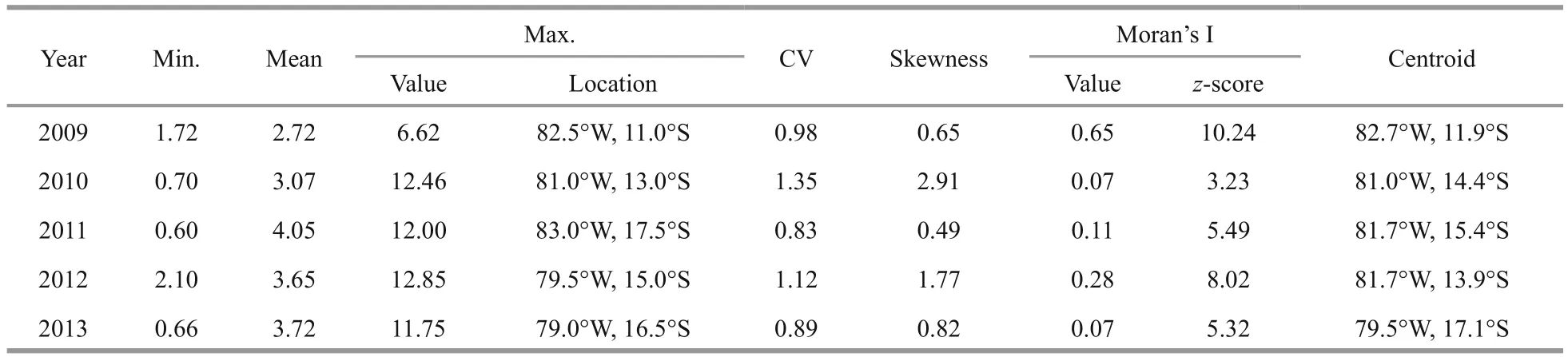
Table 1　Annual nominal D. gigas CPUE of Chinese squid-jigging fishery offshore Peru averaged over October to December from 2009 to 2013

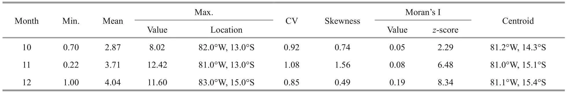
Table 2　Monthly nominal D. gigas CPUE of Chinese squid-jigging fishery offshore Peru averaged over 2009 to 2013 from October to December

Table 3　Fitting performances of the GAM and SAR models applied to examine the CPUE-environment relationships

Table 4　The residual deviance, deviance explained, Akaike Information Criterion (AIC), adjusted R2, and P-values for all possible steps in the forward selection procedure for GAM models of D. gigas offshore Peru

3.3　CPUE-environment relationships

Five criteria were adopted to evaluate the fitting performance of the GAM and SAR models in examining the CPUE-environment relationships(Table 3). The SAR model had a higher adjustedR2but a lower AIC as compared to the GAM model,indicating a better-fi t performance for the former. The sum of squared residuals for the SAR model was smaller by 2.79, which also confi rmed its better performance. For both GAM and SAR models, the sum of residuals and the Moran’s I values with relatively highP-values were close to zero, indicating random distributions of residuals for the two models.

Most of the GAM factors were statistically significant (P＜0.05) except the latitude (withP＜0.1)(Table 4). The total variance explained by the GAM model with all covariates was 31.20%, of which the month variable accounted for the highest deviance(35.31; 11.01%), the longitude accounted for the second largest amount of variance (18.07; 5.64%),and the fi shing year was the third in importance(14.43; 4.50%). Latitude corresponded with the lowest deviance (5.7) and only accounted for 1.78%of the total explained variance. The results indicate that the CPUE ofD.gigasoffshore Peru was significantly affected by month, longitude and year as inferred from the GAM model, while the impact of latitude on the CPUE was weak. The CPUE was closely related to the environmental variables of SST,SSS and SSH (in descending order ofimportance),temporal variables of month and year, and spatial variables of latitude and longitude (Fig.4). High CPUE rarely occurs north of 15°S, despite the observation that the highest CPUE for October and November were found there. With regard to the effects of temporal variables, high CPUE was observed in 2011 and December, confi rming the results presented in Tables 1 and 2.

Fig.4　Relationships between D. gigas CPUE and predictor variables derived from the GAM with 95% confi dence intervals

The spatial effects were incorporated into the model through spatial autocorrelation (Eq.4) while the longitude and latitude were included in the SAR model as explanatory variables (Table 5). All explanatory variables in the SAR model were statistically significant (P＜0.05) except longitude whoseP-value is 0.125 8, showing a similar result as the GAM model. The variation between the coeffcients indicated different effects of the variables on CPUE. The CPUE shows relatively strong positive correlations withW_ln(CPUE) (i.e. the spatially lagged version of logarithmic CPUE) and year, weak positive correlations with SST, SSH, month and longitude, and negative correlations with SSS and latitude (Table 5). This indicates that the CPUE was significantly affected by SSS, year,W_ln(CPUE) and latitude, and the order differed greatly from that of GAM.

Table 5　Summary statistics of SAR parameter estimates

3.4　Predicted monthly spatial distributions

Monthly spatial distributions ofD.gigasoffshore Peru from October to December were predicted using both the GAM and SAR models (Fig.5). The results were similar to the observed patterns for nominal CPUE when averaged over 2009-2013 (Fig.2).Specifically, the average predicted CPUE (Table 6)from both models was larger than the observed (c.f.Table 2), whereas CPUE from SAR was slightly higher than that of GAM for all three months.Excluding the GAM result for December, all skewness values were positive and suggested left-skew distributions of predicted CPUE for both GAM and SAR models. The Moran’s I values of predicted results were much larger than those that were observed, illustrating the more clustered spatial patterns of the former. The highest CPUE predicted by both models was far greater than that observed for all three months (Table 6 and Table 2). The locations of the predicted highest CPUE were displaced from the observed ones, whereas the longitudinal and latitudinal centroids of predicted CPUE were proximal to those observed for all months.

Fig.5　Predicted monthly spatial distributions of D. gigas offshore Peru using the calibrated GAM and SAR models

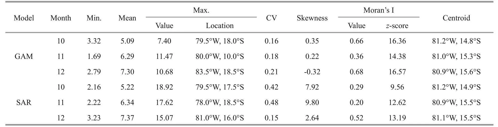
Table 6　Summary statistics of predicted monthly CPUE for D. gigas offshore Peru

Fig.6　Distributions of CPUE hotspots generated by the GAM and SAR models

The hot and cold spots of the CPUE forD.gigasoffshore Peru were calculated using Anselin Local Moran’s I (Anselin, 1995, 2004), based on the predicted results of the two models. The observed CPUE hot and cold spots were computed to produce an overlay map with the predicted CPUE hot and cold spots (Fig.6). Seven categories of the overlay maps were produced, including (1) hot-hit: hit for hotspots,(2) hot-miss: miss of hot spots, (3) hot-false: false alarm for hotspots, (4) cold-hit: hit for cold spots, (5)cold-miss: miss of cold spots, (6) cold-false: false alarm for cold spots, and (7) other types: neither hot spots nor cold spots. Visual inspection shows a clear difference between the patterns produced by the GAM and SAR models for October, whereas there are similar patterns between the two models for November and December. As inferred by the results of GAM,there was a large area of hot spots to the east of 83°W and a large area of cold spots to the west of 83°W for October. As suggested by the SAR model, there was only a small area of hot spots to the southeast and no cold spot in the entire study area. For November and December, hot spots were observed to the east of 81°W and the south of 15°S while cold spots were observed at the west of 83°W and north of 15°S, as suggested by both models.

The overall accuracy of the hotspots predicted by SAR was much better than those predicted by GAM for all months. We attribute this to SAR’s ability to correctly predict areas as non-hot and non-cold spots(correct due to other types; Table 7). Compared with the GAM model, the SAR model was less able to capture the areas containing hot and/or cold spots(HitOT; Table 7). For all three months, the SAR model hit fewer and missed more hot and cold spots but generated fewer false alarms as compared with GAM (Table 7).

Table 7　Accuracies and errors (%) of the predicted hotspots between the GAM and SAR models

4　DISCUSSION

significant interannual and monthly variability in the distribution and abundance ofD.gigasoffshore Peru was identified based on the Chinese mainland squid-jigging fishery and remotely sensed oceanographic factors (Figs.1, 2; Tables 1 and 2).Most of these important factors can be measured using remote sensing and therefore facilitate analysis of relationships between CPUE and oceanographic parameters (Valavanis et al., 2008; Wang et al., 2010;Tseng et al., 2013). However, remote sensing datasets are not perfectly continuous in time and space and may miss key data. We found that Chl-aproduction from remote sensing missed a large percentage ofinformation in the region offshore Peru from 2009 to 2013. Although spatial interpolation can estimate the missing data (Chun and Griffth, 2013), estimated data are not as reliable as observations and may result in misleading relationships between CPUE and Chla. Literature shows that the effect of Chl-aon the distribution ofD.gigasoffshore Peru is very weak(Hu et al., 2009). For the above reasons, we did not use the incomplete Chl-adata offshore Peru and focused on SST, SSS and SSH.

Annual latitudinal migration of the centroid of about 5.2°, from 11.9°S to 17.1°S, was observed forD.gigaswhile the longitudinal movement of the centroid of about 3.2°, from 79.5°W to 82.7°W (Table 1). This indicates that the longitudinal centroids were mainly located around 81°W. Earlier research showed thatD.gigasinhabit widely along the coast and its highest concentrations occurred along the coast of northern Peru from 3°24′S to 9°S during 1991-1999(Taipe et al., 2001). Our results showed that the highest concentrations ofD.gigasoccurred from 11°S to 17.5°S in recent years during 2009-2013,indicating a southward movement over time. Such a change of biological processes and distribution may be closely related to global ENSO events and dramatic changes in oceanographic conditions along the Peruvian coast (Taipe et al., 2001; Ichii et al., 2002;iquen and Bouchon, 2004).

Monthly latitudinal centroid migration of about 1.1°, from 14.3°S to 15.4°S, was observed forD.gigascompared to the longitudinal movement of about 0.2°, from 81.0°W to 81.2°W, indicating that the squid were spatially more stable and moved less on a monthly basis as compared to their annual movement(Tables 1 and 2). As suggested by both models,monthly latitudinal centroid migration was about 0.6°while latitudinal centroid migration was about 0.6°,similar to the observed migrations. Moran’s I values showed that annual spatial pattern ofD.gigasoffshore Peru was highly variable from 2009 to 2013 while the monthly spatial pattern was increasingly clustered during the peak season from October to December(Table 2).

The GAM model demonstrated the ability to identify preferred oceanographic conditions of pelagic species habitat (Ciannelli et al., 2008; Murase et al., 2009; Tseng et al., 2013). Based on the GAM model, the preferred ranges ofD.gigasoffshore Peru are SST of 20.9-21.9°C, SSS of 35.16-35.32 and SSH of 27.2-31.5 cm between 78-80°W and 82-84°W and 15°-18°S (c.f. Figs.1, 2, 4). The SAR model focused on identifying the signifi cance of each oceanographic factor and incorporated the spatial characteristics of CPUE and oceanographic factors(Table 5). The relationships between squid distribution and environmental factors may reliably reflect the distribution of the pelagic species (Yu et al., 2016b)and consequently could be used to construct models for predicting future spatial distribution patterns(Alabia et al., 2015; Igarashi et al., 2017).

Both models consider spatial characteristics in identifying the preferred oceanographic conditions ofD.gigas. The GAM model adopted longitude and latitude as the explanatory variables and examined their effects on the distribution ofD.gigasCPUE offshore Peru. In contrast, the SAR model adopted not only longitude and latitude but also the spatial relations (as reflected by spatial autocorrelation) and spatial weights (Anselin, 1980; Lichstein et al., 2002)to examine their relationship withD.gigasCPUE offshore Peru. A unique characteristic of the SAR model is its use of CPUE as both an explained and exploratory variable, which makes it autoregressive.As a consequence, the SAR model suffciently addressed the spatial characteristics of oceanographic conditions and CPUE, which in turn facilitated the identifi cation of spatiotemporal distribution forD.gigas.

From the spatial autocorrelation perspective, both hot and cold spots are strongly spatially clustered fi shing grounds with high fi shing activity, whereas the other regions showing random or non-clustered distributions are not spatially clustered (Feng et al.,2017). As such, the ability to capture hot and cold spots with less false alarms can be used to predict the distribution of pelagic species (Feng et al., 2014a; Yu et al., 2016b). Although the overall accuracy of the SAR model was greater, the model did not perform better in every aspect when compared with GAM.GAM tended to predict more hot spots than the SAR model, resulting in more false alarms of the former but more missed hot and cold spots of the latter (c.f.Fig.6 and Table 7). It is notable that both models predicted larger areas of hot spots for all three months(c.f. Fig.6) because the Moran’s I values indicating the extent of clustering and/or dispersion were larger than the observed (Table 6). Additionally, we adopted only three factors (SST, SSS and SSH) to build the models. Other important factors such as Chl-a, coastal upwelling, ENSO and oxygen minimum zone were not considered, which may lead to limitations of the calibrated models. Overall, both the GAM and SAR models appear to be valuable in predicting spatiotemporal distribution patterns and the central fi shing grounds forD.gigasoffshore Peru, based on the knowledge of CPUE-environment relationships.

5　CONCLUSION

We examined the spatiotemporal distributions and the CPUE-environment relationships forD.gigason the important fi shing grounds located between 78°-86°W and 8°-20°S offshore Peru for the Chinese squid-jigging fishery from 2009 to 2013. The GAM and SAR models were used to examine the CPUE-environment relationships forD.gigasoffshore Peru and predict the CPUE patterns from October to December. Both models predicted the spatial distributions of CPUE with considerably high accuracy. While the SAR model was more accurate, it did not outperform the GAM model in every aspect,and thus SAR cannot completely replace GAM. Our results contribute to a better understanding of spatiotemporal distributions of CPUE and the effects of environmental conditions onD.gigasin the waters offshore Peru region. By integrating fishery data and remote sensing data, modern techniques and models can be useful in identifying the spatiotemporal distribution of fi sheries and the preferred environmental conditions for pelagic species habitats.Future work should examine the impact of spatial scale on the CPUE-environment relationships forD.gigasoffshore Peru.