
Highly Efficient and Accurate Spectral Approximation of the Angular Mathieu Equation for any Parameter Values q
2018-08-06 06:10HaydarAlandJieShen
Journal of Mathematical Study 2018年2期
Haydar Alıcıand Jie Shen
1Department of Mathematics,Harran University,63290 S¸anlıurfa,Turkey;
2Department of Mathematics,Purdue University,47907 West Lafayette,IN,USA.
Abstract.The eigenpairs of the angular Mathieu equation under the periodicity condition are accurately approximated by the Jacobi polynomials in a spectral-Galerkin scheme for small and moderate values of the parameter q.On the other hand,the periodic Mathieu functions are related with the spheroidal functions of order±1/2.It is well-known that for very large values of the bandwidth parameter,spheroidal functions can be accurately approximated by the Hermite or Laguerre functions scaled by the square root of the bandwidth parameter.This led us to employ the Laguerre polynomials in a pseudospectral manner to approximate the periodic Mathieu functions and the corresponding characteristic values for very large values of q.
AMS subject classifications:33E10;33D50;65L60;65L15
Key words:Mathieu function,spectral methods,Jacobi polynomials,Laguerre polynomials.
1 Introduction
Mathieu functions were first introduced by Mathieu in 1868 while investigating the vibrating modes of an elliptic membrane[32].The eigenpairs of the Mathieu equation are needed in many scientific phenomena including wave motion in elliptic coordinates such as acoustic and electromagnetic scattering from an elliptic structures[14,19,26,31],particle in a periodic potential[22]and vibrational spectroscopy of molecules with near resonant frequencies[37,43].Theoretical aspects of the Mathieu functions have been studied by many authors,including Stratton[42],McLachlan[33],Sips[41],Meixner&Sch¨afke[34]and Wang and Zhang[45](cf.also[44]).
As is seen for many physical and mathematical problems in elliptic geometries the separation of variables process in elliptic coordinates leads to the Mathieu equations.If one wants to solve these problems with large wavenumbers,it is very important to be able to obtain accurate numerical solutions for the angular Mathieu equation for very large values of q since it is related to the wavenumber parameter present in these equations.
Mathieu functions remain difficult to employ,mainly because of the impossibility of analytically representingthemin asimple and handyway[41].Thereare numerousstudies on the numerical computation of the Mathieu functions and corresponding eigenvalues.Erricolo used Blanch’s algorithm for computing the expansion coefficients of Mathieu functions[16].Erricolo and Carluccio provided software to compute angular and radial Mathieu functions for complex q values[17].Shirts presented two algorithms for the computation of eigenvalues and solutions of Mathieu’s differential equation for noninteger orders[39,40].Alhargan introduced algorithms for the computation of all Mathieu functions of integer order which can deal with a range of the order n(0−200)and the parameter q(0−4n2)[3].Co¨ısson and co-workers describe a numerical algorithm which allows a fl exible approach to the computation of all the Mathieu functions[12].Cojocaru in[13]provided Mathieu functions computational toolbox implemented in Matlab.MATSLISEis anothersoftware package for the computationof the Mathieu eigenpairs by using the power of high-order piecewise constant perturbation methods[29]and many others[1,9,21,24,25,28,30].
Most of the above algorithms employ the well-known trigonometric series representation
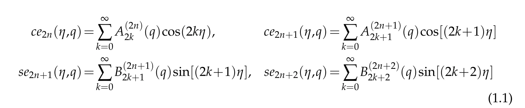
forcomputingtheperiodicMathieufunctionswhere A and B are knownas theexpansion coefficients.There are several ways of computing these expansion coefficients such as continued fractions method[33],the forward and the backward recurrence relations[9,17]and as the eigenvectors of tri-diagonal matrix-eigenvalue problems[12,13].Each has its advantages and disadvantages.However,these algorithms are not suitable for very large values of q.Thus,the aim of this study is to construct accurate and efficient spectral algorithms for the computation of the integer order periodic Mathieu functions and the corresponding characteristic values for both small and very large values of the real parameter.
The rest of the paper is organized as follows:Sections 2 and 3 are concerned with the construction of the spectral methods for small and very large values of q,respectively.Some numerical results are presented in Section 4.The last section concludes the paper with some remarks.
2 Spectral formulation for small and moderate parameter values
For any given value of the parameter q,the angular Mathieu equation

supplemented with a certain periodic boundary conditions admits two linearly independent families of periodic solutions with period π or 2π for specific values of the separation constant λ.Such values of the parameter λ are known as characteristic values or eigenvalues.When the solutions Φ(η)are even with respect to η =0 the characteristic values are denotedas an(q)whereas for odd solutions they are representedas bn+1(q),n=0,1,....Periodic eigenfunctions corresponding to the an(q)and bn+1(q)are denoted by cen(η;q)and sen+1(η;q),respectively.Thenotations ce and se are dueto Whittakerand Watson[47]and they stand for cosine-elliptic and sine-elliptic,respectively.Before describing the nu-

Table 1:The periodic Mathieu functions.
merical scheme,we firsttransform theangular Mathieuequationto a more tractable form for each boundary condition set in Table 1.The angular Mathieu equation in(2.1)and Table 1 allow us to write

that can be transformed to an equivalent algebraic form

by the mapping x=cos2η∈(−1,1)where yn(x;q)=ce2n(x;q).The connection formula

reveals that the function y does not have to satisfy any boundary conditions at all.Next,we consider the system

and have found the corresponding algebraic form to be

upon use of the transformations x=cos2η and ce2n+1(x;q)=(1+x)1/2yn(x;q)on both independent and dependent variables,respectively.Returning back to the original variables we see that the solution

satisfies the boundary conditions in(2.5)meaning that we don’t need to impose any boundaryconditionson(2.6).Thirdly,themaps x=cos2η and se2n+1(x;q)=(1−x)1/2yn(x;q)transform the system
to the equivalent algebraic form
without any boundary conditions since the solution

readily satisfies the conditions in(2.8).Finally,the system

can be converted to the form

by means of x=cos2η and se2n+2(x;q)=(1−x2)1/2yn(η;q).Again,the solution in original variable

satisfies the specified boundary conditions.
Actually the equations in(2.3),(2.6),(2.9)and(2.12)can be put together to give the equation

with
体育和其它文化课程的区别是体育课是为了促进学生身心健康发展的辅助性课程,它的教学目的不是为了让学生取得高成绩,而是为了让学生拥有一个强健的体魄,所以体育课并没有很多死板的理论知识课程。但是传统体育教学方法只对跑跳等运动进行简单的训练,无法充分的激发起学生足够的体育热情。小学生由于心智还在萌芽发展时期,对很多事情都有着充足的好奇心但缺乏长久的耐性,小学体育游戏教学法将体育运动充分有效地融入到游戏之中,利用游戏的教学方法将枯燥的体育活动变得生动、有趣。在游戏中学生的天性和好奇心可以得到释放和满足,使小学体育教学朝着积极健康的方向不断发展。

The characteristic values

of(2.1)are connected with those of the equation in(2.14)by the relations

respectively,while the corresponding eigenfunctions

are related with the solutions of(2.14)by the formula

Notice that,the set of parameter valueslead to the eigenpairs(ce2n,a2n),(ce2n+1,a2n+1),(se2n+1,b2n+1)and(se2n+2,b2n+2),respectively.Here,the constant C will be chosen in such a way that||Φ(η;q)||L2(0,π)=π.That is,

leading to
when the orthonormal eigenfunctions||yn||L2ω(−1,1)=1 of(2.14)is in consideration.
Now,we will construct the Galerkin spectral formulation of(2.14).Let


The Spectral-Galerkin method for(2.14)is to findsuch that

where ω(α,β)(x)=(1−x)α(1+x)βis the Jacobi weight function.Now,proposing
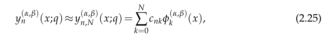

we see that the Spectral-Galerkin formulation(2.24)of the differential eigenvalue problem(2.14)reduces to the matrix-eigenvalue equation

with cn=(cn0,cn1,...,cnN)T,S=[Sjk]=−k(k+α+β+1)δjkand

The three term recurrence relation of the normalized Jacobi polynomials
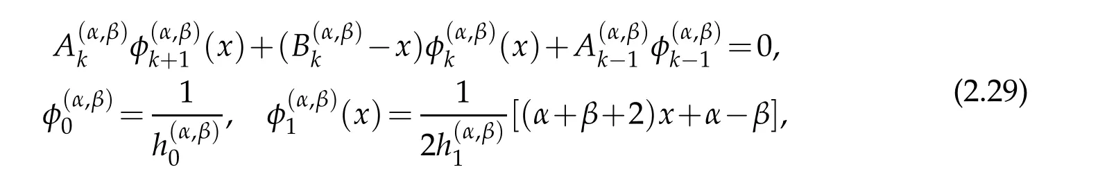
in which
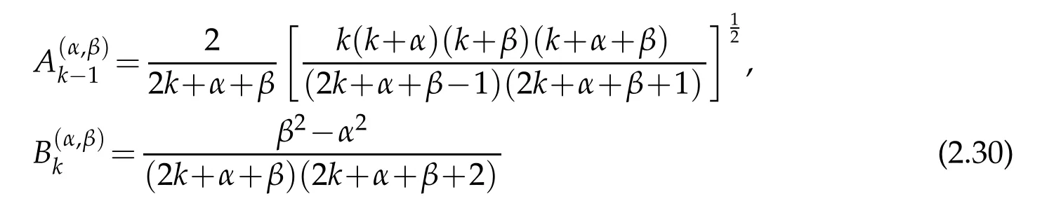
allows us to write down the entries
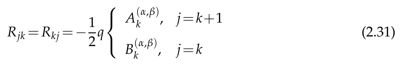
ofthesymmetrictri-diagonal matrix R for j,k=0,1,...,N.Noticein(2.31)that thediagonal entries are all zero since we havefor all k whenMoreover,the entries of the matrix R requires special attention whensince in this case the first coefficient
The matrices have simple structure,more specifically S is a diagonal and R is a tridiagonal matrix with zero main diagonal.Thus,the resulting discrete system is a tridiagonal matrix.Despite its simple structure,the present formulation yields highly accurate numerical eigenpairs.For small q values,even the last discrete eigenpair corresponding to N is correct up to some digits which is promising if we remember the fact that only the two-thirds,often one-half or considerably smaller portion of the computed eigenpairs are correct up to some accuracy for a fixed truncation order N[10,46].Speci fically,when q=1 and N=100,relative errors for all the eigenvalues except the last one are of order 10−14and for the same N with q=102,ninety-four of them have relative errors of order 10−14.

Table 2:The number of eigenvalues(ev)having relative errors of order 10−14and the number of eigenvectors(ef)having absolute errors of order at most 10−13for a given truncation order N and the parameter q.
On the other hand,the number of accurate aigenvectors having the values of the Mathieu functions at some evaluation points is slightly less than that of eigenvalues.The accuracy of the eigenpairs are checked by increasing the truncation order N systematically and observing the stable digits between two consecutive truncation orders N and N+1.For the eigenvectors,vector infinity norm is used to measure the errors.
Nevertheless,it can be seen from Table 2 that the number of accurate pairs decreases with a further increment in q.Indeed,a dramatic decrease occurs especially for q≥105.Therefore,in this article such q values will be called very large.Actually,the accuracy loss for large values of the parameters is typical for all parameter dependent problems such as the Coffey-Evans[18]and the prolate spheroidal wave equation.Efficient numerical approximation of the latter for very large values of the bandwidth parameter may be found in[4,27,35].An efficient method for very large values of the parameter q will be derived in the next section.
3 Spectral formulation for very large parameter values
The main difficulty for very large q values originates from the fact that the eigenfunctions of(2.1)are confined to a small interval around the points η=π/2 and η=3π/2 whenthey are considered in the interval(0,2π)(see Figure 1).Therefore,one has to focus on these portions of the interval.One remedy might be the use of mapped Jacobi pseudospectral methodsby using a suitable mapping suchas the one introducedin[7]which can clusters more points around a desired point.However,here we are in favor of employing another technique which is more efficient and accurate from the numerical point of view.
Consider the general equation
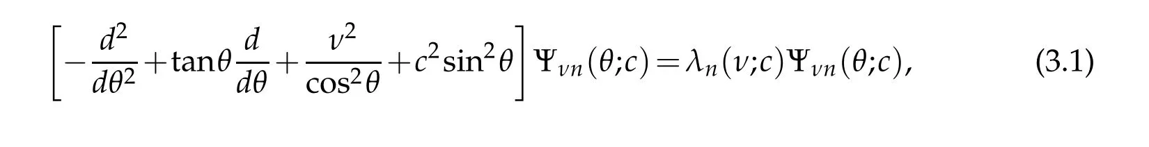
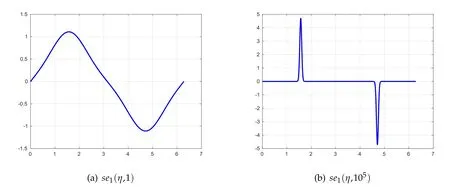
Figure 1:se1(η,q)for specified values of q on[0,2π].
where c and ν>−1 is a real parameter.The maps t=sinθ and Ψνn(θ;c)=(1−t2)νψνn(t;c)takes the equation to the algebraic form

where µn(ν;c)=ν(ν+1)−λn(ν;c).Stratton[42]and later Chu and Stratton[11]defined the spheroidal functions as the solutions of the last equation that remains finite at the singular points t= ±1.For integral orders ν=m=0,1,2,...the functions ψνn(t;c)are related to the spheroidal wave functions that arise from separation of the Helmholtz equation in spheroidal coordinates.For half-integer values ν=±12they are related to the angular Mathieu functions that arise from separation of the Helmholtz equation in elliptic coordinates[38].Thus,we may make use of(3.1)to approximate the eigenpairs of the angular Mathieu equation for very large values of q whose details will be explained below.
Note that,the solutions ψνnof(3.2)that remain finite at the end points t=±1 suggest the use of boundary conditions Ψνn(±π/2;c)=0 for(3.1).This makes equation(3.1)into a reflection symmetric system so that the even and odd states can be separated.Actually the transformations x=−cos2θ and Ψν2n(x;c)=(1−x)ν/2yνn(x)lead to the equation
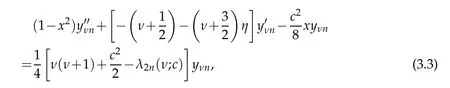
where x∈(−1,1).Onreturningback totheoriginalvariables Ψν2n(θ;c)=cosνθyνn(−cos2θ),we see that the even indexed eigenfunctions are even functions of θ.For the odd states,first we use the map Ψν2n+1(θ;c)=sinθφν2n+1(θ;c)=where φν2n+1is necessarily an even function of θ.This suggest use of the same transformations employed for the even states leading to the equation
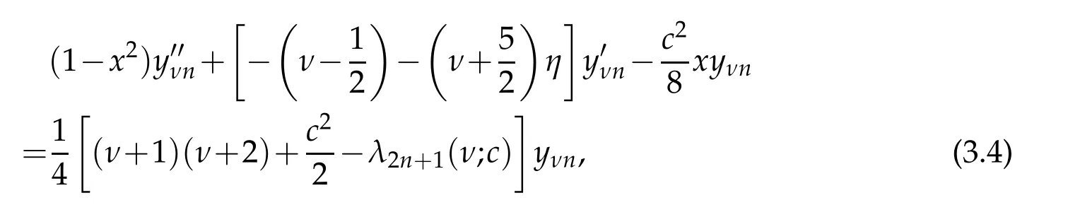
where the odd state eigenfunctions Ψν2n+1(θ;c)=sinθcosνθyνn(−cos2θ)are indeed an odd function of θ.Therefore,instead of(3.2),we have two equations to handle the even and odd states of(3.1)separately.Actually the last two equations can be unified as

in which
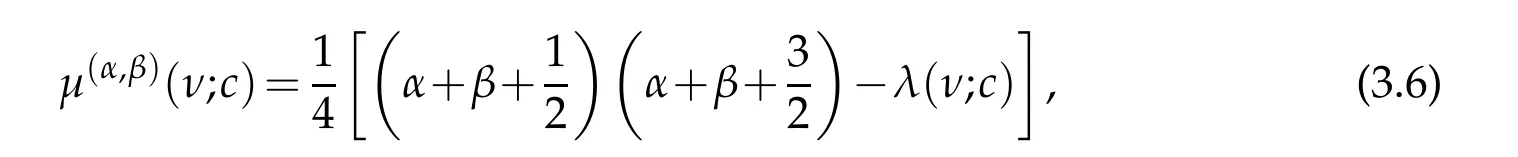
where the parameters(α,β)=(ν,−)and(α,β)=(ν,)yield the even and odd states,respectively.
Now,taking c2=4q and comparing(3.5)-(3.6)with(2.14)-(2.15)we obtain the connection relations
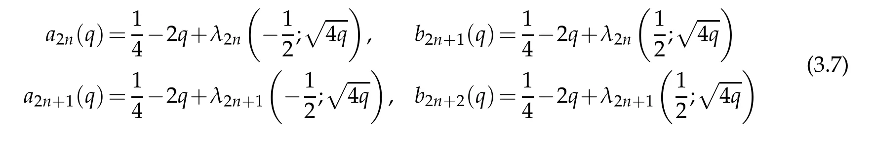
among the eigenvalues of the Mathieu and the generalized spheroidal equation in(3.1).Meanwhile,the well-known relations[33]

among the eigenvalues oftheMathieu equation,togetherwith(3.7)lead tothe interesting relations
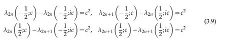
among the eigenvalues of(3.1)when ν=±1/2.
For the spheroidal wave equation,that is when ν=m=0,1,2,...in equation(3.1),we have presented highly accurate and efficient method for very large values of the bandwidth parameter c[4].It was based on the idea that when c tends to infinity,the prolate spheroidal wave functions can accurately be approximated by the Hermite functions scaled by the square root of the parameter c[6,15,20,27,36].Clearly,they can also be approximated by the Laguerre functions of order±due to the connections

between the Hermite and Laguerre polynomials.The same idea can be used with ν=±to approximate the eigenpairs of the Mathieu equation as well.To this end,we transform the equation in(3.1)to another one over the positive half line.This can be accomplished by the maps

and

applying in respective order.The first map leads to the operational equivalence

for the differential part of(3.1)which is not the case for the operator d2/dη2present in the angular Mathieu equation in(2.1).That is to say,in this case it is not possible to find a transformation from the interval η ∈(0,π/2)to the half line x∈(0,∞)leading to such an operator with linear and constant polynomial coefficients.That is why we make use of the more general equation in(3.1)and finally take ν= ±since in these two cases the solutions of(3.1)are related with the angular Mathieu functions.Application of the above transformations lead to the equation

where
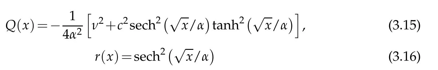

from which we can compute the characteristic values of the Mathieu equation employing the connection formula(3.7)with ν=and c=p
Here,α is a scaling or an optimization parameter whose optimum value is usually determined by trial and error.However,fortunately,for this problem as is explained above its optimum value is fixed as αopt==(4q)1/4.To approximate the eigenpairs of(3.14),we utilize the Laguerre functions in a pseudospectral picture since it reduces to the differential equation for the Laguerre functions when q(x)≡0 and r(x)=1.Basically,the idea is to collect the grid points,that are the roots of the order γ=±1/2 Laguerre polynomials,to the small interval where the eigenfunctionsare away from zero by means of the scaling factor αopt=.Now,consider the weighted interpolation of the solution of(3.14)

in which
are the set of N−th degree Lagrange polynomials and xkstand for the N+1 real and distinct roots ofwhich are computed by using the well-known Golub-Welsch algorithm[5,23].Proposingthe interpolant as an approximate solutionto(3.14)and requiring the satisfaction of(3.14)at the collocation points xk,we obtain a discrete representation

where Q(xn)are the values of the function Q(x)in(3.15)at the nodal points xn.This matrix can be factored asˆB=SBS−1where S=diag{s1,s2,...,sN}is diagonal matrix with

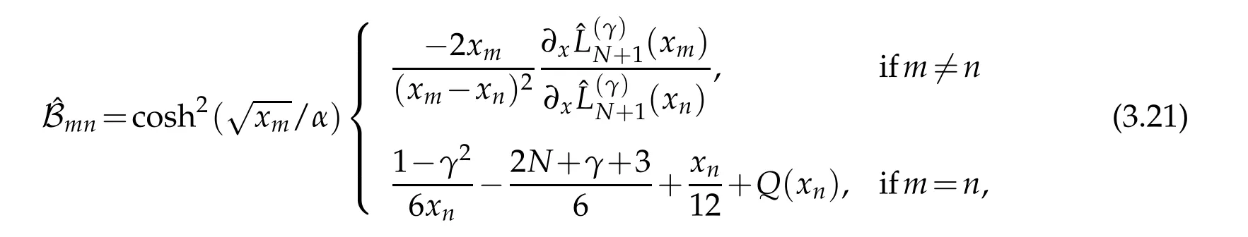
and B is symmetric matrix with entries

Therefore we may replace the unsymmetric system in(3.20)with the symmetric one

since the similar matrices share the same eigenvalue set.Clearly,an eigenvectorof(3.20)is connected with that of(3.24)by

On the other hand,for an orthonormal eigenfunction of(3.14)we may write

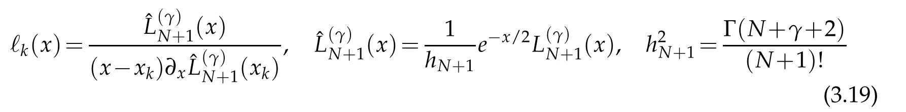
where we have used(3.12).However,applying the change of variable sinθ=tanhin(3.11),to an eigenfunction of(3.1)we obtain


of the normalized Laguerrefunctions in(3.19)with n=N+1 and x=xk,we may represent the angular Mathieu functions in terms of the spheroidal functions of orders ν=±1/2 as
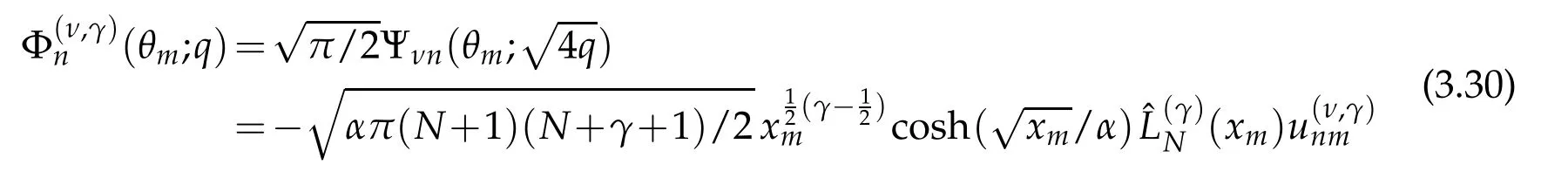

where

The matrix in(3.23)only necessitates the knowledge of the zeros of the(N+1)−st degree Laguerre polynomial of order γ=±1/2.It is easy to construct and symmetric with quite reasonable condition number.In fact,numerical experiments reveal that as q gets larger,the condition number of the matrixBof size(N+1)×(N+1)converges to 4N+1 and(4N+3)/3 when γ = −1/2 and γ =1/2,respectively.
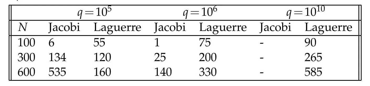
Table 3:The number of eigenvalues having relative errors of order 10−14for a given truncation order N and the parameter q.
Now,in Table 3 by comparing with the Jacobi spectral method we see that the Laguerre pseudospectral formulation leads to much better results for large q values,especially as q gets larger and larger.
4 Numerical results
In this section we present some numerical tables and plots of eigenfunctions for small,moderate and very large values of the parameter q.
It is clear from Table 4 that the algorithms mentioned in this study can accurately approximate the eigenvalues when the parameter q is small.Here we executed our algorithm in Fortranquadruple precisionarithmetic to see if the results agree with thoseof[1]up to the accuracy quoted.This does not mean that the other algorithms can not attain such accuracy for small q.In contrast,there would have been algorithms cited in this study which can also attain the same accuracy if they were implemented in quadruple precision arithmetic,too.
Then in Table 5 we present the discrete values of the function ce9(η,100)at the specified angles.First two columns include the results obtained from the present Jacobi-Galerkin method with the truncation orders N=25 and N=26.The last column includes the results from[8]which truncates the second series in(1.1)at N=20.Although it seems that,our method yields better results then the classical trigonometric series expansion,at a cost of computing more expansion coefficients,the trigonometric series can also produce results that are accurate to machine precision.It is clear from Table 5 that for small values of q both the present Jacobi-Galerkin and the trigonometric series approach produce similar results.

Table 4:Comparison of b2(25)and b10(25)with some literature results.

Table 5:Values of the Mathieu function ce9(η,100)at the specified angles η.
Table 6 demonstrates the accuracy improvement of b2n+1(q)for the parameter values q=1,1010and eigenvalue indices n=1,1001.It is clear that the methods described here not only yield accurate results for lower states,but also for higher ones as high as thousand with quite reasonable truncation orders N.As a result of separation,the necessary truncation size to print b1001(1)on the screen is N=501.However,N=502 is enough to obtain it with a relative error of order 10−15.Similarly,N=513 does the same job for b1001(1010)revealing the efficiency of our algorithms.
For comparison,the bottom row includes the results obtained from MATSLISE package[29]and Cojocaru[13].The latter diagonalizes the tri-diagonal matrix resulted from writing the recurrence relation of the expansion coefficients of(1.1)in matrix form.As it is mentioned in Introduction,this type of approaches are suitable for small or moderate q values and not able to produce satisfactory results for very large values of the param-eter q.Specifically,N=2000 was not enough to approximate the eigenvalue b1001(1010).Even for the ground state eigenvalue b1(1010)one needs to diagonalize a matrix of size N=1100.Actually,MATSLISE works for very large values of q as high as 1013beyond which it also has difficulties in approximating the Mathieu eigenpairs.

Table 6:Accuracy improvement for b1001(q)for q=1 and q=1010by using the Jacobi and the Laguerre bases,respectively.
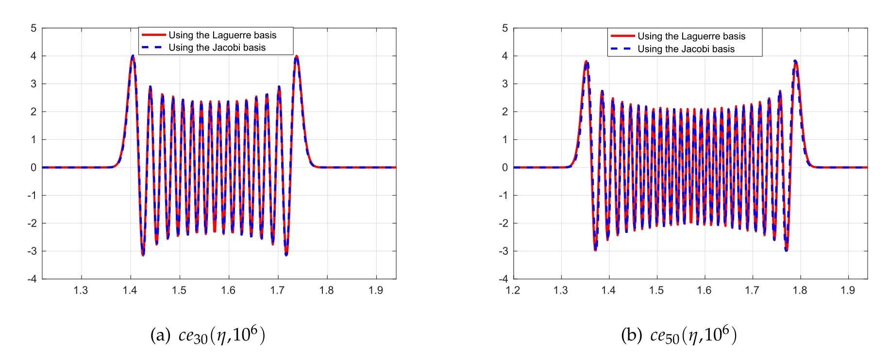
Figure 2:ce30(η,106)and ce50(η,106)corresponding to the characteristic values a30(106)=−1878467.04186782 and a50(106)=−1799283.43142027,respectively.
For large values of q it is still possible to approximate the lower eigenpairs by the Jacobi bases at a cost of very high truncation orders.In Figure 2 we present plots of the Mathieu functions ce30(η,106)and ce50(η,106)that are obtained by using both the Jacobi and the Laguerre bases.Note the confinement of the eigenfunctions to a small interval around the point π/2 for such large values of q.
In order to check the efficiency of the Laguerre basis approach,in Table 7 we include several eigenvalues for very large value of q=1020.In this case,the integer part of the eigenvalues occupy more than twenty digits.Therefore,we have implemented our algorithm in Fortran programming language by using quadruple precision arithmetic and tabulate the values a(q)+2q or b(q)+2q instead of a(q)and b(q),respectively.To approximate the eigenvalue a1000(1020)with the present Laguerre pseudospectral methodto the accuracy quoted,we only need to diagonalize a matrix of size 505×505 which is impressing.It is known that,for finite n and large q values a2n(q)≈b2n+1(q)and a2n+1(q)≈b2n+2(q)[33].This can also be observed from the equations(3.14)-(3.16)and(3.7).In fact,in(3.14)one has λn(ν,c)=λn(−ν,c)since there is a quadratic dependence on ν.Then,it is easy to see that an(q)≈ bn+1(q)by employing this fact in the connection formulas(3.7).Numerical results in Table 7 are in accordance with the asymptotic formula
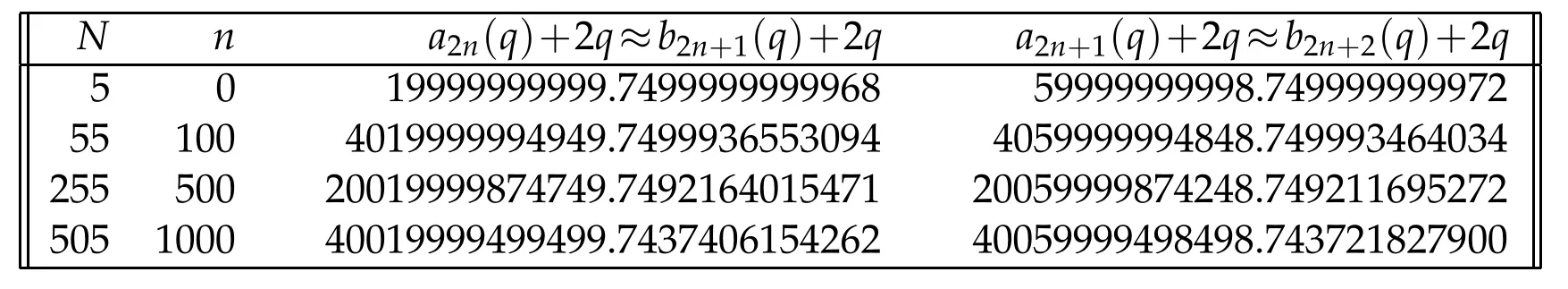
Table 7:Several eigenvalues of the angular Mathieu equation for q=1020.
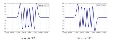
Figure 3:Mathieu functions ce10(η,q)and se12(η,q)corresponding to the characteristic values a10(q)+2q=419999999944.7499999927156 and b12(q)+2q=459999999933.7499999904406,respectively.
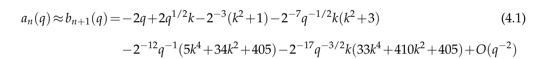
up to their last digits where k=2n+1[28,33].
Then,in Figure 3 we present the plots of two eigenfunctions corresponding to the same q=1020.Notice in this case that their nonzero parts are confined to a tiny interval of length 10−4around the points(2k+1)π/2 where k is an integer.
5 Conclusion
In this article,we have constructed accurate and efficient spectral and pseudospectral methods based on the Jacobi and the Laguerre polynomials to approximate the integer order periodic Mathieu functions and the corresponding characteristic values.To this end,the angular Mathieu equation is transformed into several equations resembling the Jacobi and the Laguerre differential equations.These particular transformations motivated us to use the most suitable Jacobi or Laguerre polynomial with specific parameter(s)as basis sets for the approximation of the eigenpairs.It is observed from numerical results that the Jacobi-Galerkin methods are well suited for small q values whereas the Laguerre pseudospectral methods scaled by(4q)1/4are more appropriate for very large values of q.Note that,in the Laguerre pseudospectral method a suitable scaling parameter optimizing the accuracy is not chosen by experimentally since it is initially set as αopt=(4q)1/4.
The algorithms developed in this paper are implemented in a set of Matlab routines,Mathieu.m,Mathieu_Small_q.m,Mathieu_Large_q.m and eigfunplot.m,which can be downloaded via the link http://www.math.purdue.edu/~shen/pub/mathieu.zip.The routineMathieu.mservesas themain filewhichcalls theotherthreetocomputetheMathieu eigenpairs.Mathieu_Small_q.mand Mathieu_Large_q.mapproximate the eigenpairs for|q|<106and|q|≥106,respectively whereas Eigfunplot.m is responsible for plotting the results obtained from these routines.
The methods developed here will be useful in a variety of physical and engineering applications in which accurate solutions of the angular Mathieu equation are needed.
6Acknowledgement
The first author’s research was supported by a grant from T¨UB˙ITAK,the Scientific and Technological Research Council of Turkey.The second author’s research was partially supported by NSF DMS-1620262,DMS-1720442 and AFOSR FA9550-16-1-0102.
猜你喜欢
甘肃教育(2020年2期)2020-09-11
小学教学研究(2019年25期)2019-09-08
小学生优秀作文(低年级)(2019年5期)2019-04-25
养生保健指南(2017年1期)2017-02-08
党员干部之友(2016年10期)2016-02-01
体育师友(2015年3期)2015-12-22
散文百家(2014年11期)2014-08-21
中国学校体育(2014年11期)2014-05-10
体育师友(2011年2期)2011-03-20
中国校外教育(上旬)(2006年5期)2006-05-25
 Journal of Mathematical Study2018年2期
- Journal of Mathematical Study的其它文章
- Ill-posedness of Inverse Diffusion Problems by Jacobi’s Theta Transform
- POD Applied to Numerical Study of Unsteady Flow Inside Lid-driven Cavity
- Generalized Hermite Spectral Method for Nonlinear Fokker-Planck Equations on the Whole Line
- A Diagonalized Legendre Rational Spectral Method for Problems on the Whole Line
- Chebyshev Spectral Method for Volterra Integral Equation with Multiple Delays