Numerical study of steady-state acoustic oscillations in semi-closed straight channel *

Dinar Zaripov

Institute of Power Engineering and Advanced Technologies, FRC Kazan Scientific Center, Russian Academy of Sciences, Kazan, Russia

School of Mechanical Science and Engineering, Huazhong University of Science and Technology, Wuhan 430074,China

Abstract: The influence of properties of finite-difference schemes of Godunov, Lax-Wendroff and TVD on prediction of amplitudefrequency responses of pressure oscillations is investigated as a part of a problem of steady-state oscillations in a semi-closed channel.Problems of Riemann and pipe draining are solved as a test. It is shown that the dissipative properties of Godunov scheme underestimate the amplitude of high-frequency oscillations relative to the experimental data. Lax-Wendroff scheme predicts an amplitude-frequency response with sufficient degree of accuracy. TVD scheme leads to nonmonotonic amplitude-frequency response and overestimates values of resonance frequencies.

Key words: Acoustic oscillations, straight channel, resonance, finite-difference scheme

Introduction

Currently mathematical modelling along with experiment is often used in solving applied problems of hydrodynamics. The shift of attention of scientists and engineers in the direction of numerical simulation is due to the difficulties in application or even inapplicability of analytical methods. However, numerical methods lead to error in evaluation of values associated with finite-difference approximation of the original equations. Therefore the results of numerical calculations must be comprehensively inspected and tested using test problems and experimental data.

The Riemann problem[1-2]is one of the frequently used test problems. This test is attractive because there is a self-similar solution for this case. It has been first applied by Godunov et al.[2]in solution for gas dynamics equations. Another traditional test is the Shu-Osher problem[3]. It is often used to verify simulation results of unsteady processes. This problem differs from the Riemann problem in non-uniform initial distribution of thermodynamic parameters over the whole computational domain. Unfortunately,despite its simplicity, this problem is not convenient for the verification of results of unsteady viscous flows numerical modelling over large time intervals.This is because the initial perturbations are damped due to friction and absence of permanent source of forced oscillations. Study of factors affecting the quality of simulation of different flows can be often found in literature. For example, the effect of TVD-schemes with flux vector splitting on the solution for the one-dimensional advection problems is studied in Refs. [4-5]. In Ref. [5] the Riemann problem is considered as a test. It is shown that the calculation results strongly depend on the integration scheme.

Unfortunately, mathematical modelling in a large range of hydrodynamic problems is limited to investigations of the studied processes on small time scales.As a rule, this is due to limited computational resources. Meanwhile, there are problems in which the processes occurring on large time scales are investigated. For example, settling of a shock-wave pattern when a supersonic under expanded jet impinging on a plane obstacle is shown in Ref. [6] in the context of simulation of dynamics of the unsteady flow around bluff bodies on large time scales. The need to study this problem over large time intervals is associated with the long-term development of the periodic auto-oscillatory process. As noted in Ref. [6], to verify the obtained numerical data, special tests are required in addition to traditional testing. The evolution of pollutant concentration in the River Thames estuary on time scales of about two days is considered in Ref.[7]. The second order accuracy MacCormack explicit scheme was used in this work. It was noted that the solution of the model problem over the time interval of a few minutes leads to deviation of the obtained values from the exact solution. In addition, TVD scheme enables one to reduce numerical diffusion.Nevertheless, the data obtained using numerical schemes should be verified with known experimental data and compared with the exact solutions to model problems.

Study of unsteady processes in a circular channel[8-10]is a characteristic problem in the research of undamped processes over large time intervals. The problem of pipe draining[8]is a classical problem in which a gas motion is induced with the help of an initial pressure differential between ambient air and cavity of the pipe. In this case, taking into account processes occurring at the open end of the pipe(inflow and jet outflow) leads to a damped periodic process in the pipe, as shown in Ref. [8]. In Ref. [9],body forces are considered to be a source of perturbation when modelling undamped oscillatory processes in a cavity of a circular channel. A piston moving at one of the channel’s boundaries is discussed in Ref. [10]. In Ref. [11], the pressure oscillations in the environment are considered to be a source of noise. The numerical implementation of this condition is discussed in Ref. [12].

One of the features of problem of steady-state oscillations is the formation of standing waves in the cavity of the channel, in which the amplitude of oscillations increases after multiple reflections of pressure waves from the boundaries of the area under consideration. This results in long-term development of the periodic oscillation process and a multiple increase of calculation time in computational modelling. However, the problem of the influence of the numerical scheme on the amplitude-frequency response of steady oscillations in semi-closed channel remains open. Since the oscillatory gas motion in a straight channel is a classic and comprehensively studied problem, it is well suited to study the influence of integration schemes on the amplitudefrequency response of flow oscillation over large time interval.

In nature, the flow in the straight channel is three-dimensional and the flow parameters such as velocity and pressure are non-uniformly distributed along the direction of the normal to the wall.Non-uniformity becomes even stronger due to the deviation of sidewall shape from axially symmetric one. Thus, in general, three-dimensional equations must be considered. In this case, the computation cost becomes extremely high when considering unsteady flow in long channels (gas pipelines, for instance)over large time interval that is not affordable.However, for long channels, more precisely, when the radius-to-length ratio of the channel tends to zero,three-dimensional phenomena are negligible and the use of averaged parameters over the channel crosssection is more relevant. Thus, one-dimensional equations might be considered in this case. This allows significant reduction of the computational time that is essential for practice.

1. Mathematical problem

Consider a problem of oscillating flow of a weightless gas in a straight circular channel closed at one end and open at the other end (as shown in Fig. 1).Suppose that the gas motion in the cavity of the channel is induced under the external source of oscillations defined by the following expression

where0p is the constant pressure in the quiescent environment, ()g t is the periodic pressure component of the environment defined in general as a sum of harmonic functions.

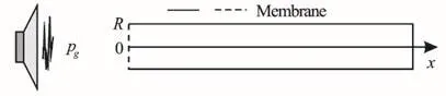
Fig. 1 Scheme of channel and location of the external source of oscillations

Assume that there is an isentropic gas flow at the channel inlet which occurs simultaneously with a pressure change in the ambient air. So the total pressure at the inlet section is determined by the Eq.(1) and, according to Bernoulli equation, the static pressure is defined by

where p and u are the static pressure and velocity at the inlet section, respectively, ζ is the drag coefficient depending on the type of the inlet section.Introduction of the drag coefficient ζ is necessary for taking into account the flow separation. Neglecting this can lead to physically incorrect results[8]. One of many problems where the drag coefficient should be taken into consideration is the pipe draining. However,in considering a free discharge from the channel, the pressure at the outlet section of the channel corresponds to the pressure in the ambient air with sufficient degree of accuracy. In this case, the quadratic term in Eq. (2) should be discarded and Eq. (1) should be employed for determining the output pressure, whereas for steady separation-free channel inflow =0ζ.

Since the isentropic flow at the interface between the channel cavity and the ambient air is considered,the temperature at the open end can be written aswhere p is the static pressure determined by Eq. (2), k is the adiabatic coefficient,and0are the temperature and pressure at the inlet section at the initial time, respectively.

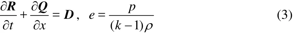
Motion, continuity, energy and state equations describing a one-dimensional flow in circular channels[11]are used

No-slip and impermeability conditions are fulfilled at the impermeable boundary (closed end). As noted in Ref. [8], real processes occurring at the open end of the channel should be taken into account when modelling the unsteady flows. The paper[12]represents a numerical implementation of boundary condition describing correctly the processes occurring at the open end of the channel. It is shown that the velocity of disturbances propagation and the static pressure values in the channel are correctly determined, too.The essence of it is as follows. The boundary condition (2) and the linearized Eq. (3) are considered

where0c is the sound velocity in the quiescent environment has a density of0ρ. Considering their finite-difference approximations, a quadratic equation to determine the velocity at the left boundary can be derived, which has the following solutions

where the upper and lower signs correspond to inflow and outflow, respectivelyis the Courant number,μ is the gas viscosity. The superscript in Eq. (5)corresponds to the values of pressure p and velocity u corresponding to the time layer n. The subscripts correspond to their values at a boundary node “0” and an adjacent inner node "1" of mesh in space. The finite-difference mesh is shown in Fig. 2. The value of the static pressure at the open boundary of the channel can be derived substituting the value of the velocity determined by Eq. (5) into Eq. (2). The initial (=0)τ values of pressure p and density ρ along the channel are constant, the initial flow velocity is equal to zero (=0)u .

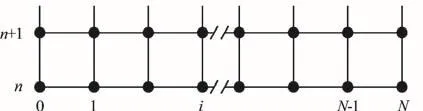
Fig. 2 Finite-difference mesh

2. Numerical scheme

In terms of studies of the effect of difference schemes’ dissipative and dispersive properties on the simulation result over large time intervals, first- and second-order schemes are the most suitable. It is known that the first-order schemes, e.g., Godunov scheme[2], have so-called numerical viscosity[1]resulting from discretization of the computational domain and approximation of differential equations by their difference analogues. This property results in the solution to differential equations with additional viscous terms and reduces the accuracy of the result.Solution smearing inherent in Godunov scheme becomes more significant on large time scales. A finite-difference Godunov scheme[1]of the first-order accuracy can also be considered. This scheme leads to solution essentially coinciding with[2]and requires significantly less computational resources. In contrast,application of second-order accuracy schemes leads to unphysical oscillations in the region of large gradients of flow parameters or the channel shape (e.g., shockwaves or sudden changes in cross-sectional area) due to dispersion properties of difference schemes. It is a consequence of the dispersion properties of difference schemes[1]. The Lax-Wendroff scheme[1]of the second-order accuracy should be noted among other second-order schemes.

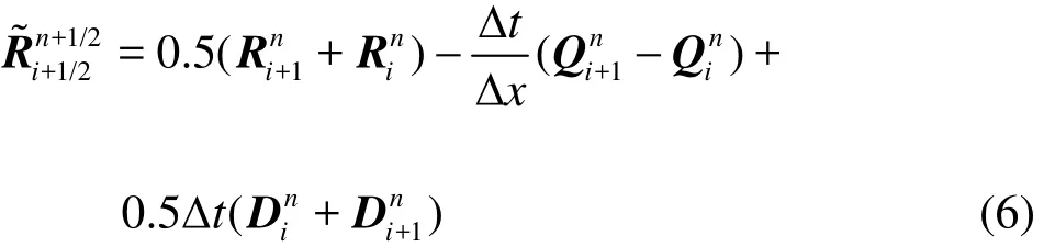
In accordance with the schemes of Godunov and Lax-Wendroff, at first, values of the grid function at half-integer points of the stencil at the intermediate layerare calculated:

Godunov scheme

Lax-Wendroff scheme

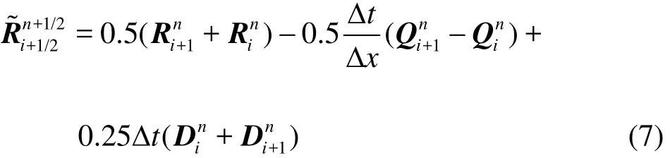
Then the solution for the top layer at the pointis calculated for both schemes

These schemes are stable under the CFL conditionwhere 01v＜≤ is the Courant number.

The TVD scheme with minmod, Van Leer, MC and superbee limiters[13]is also considered in this work. Eq. (8) is used as a TVD scheme in which numerical flux is built in the following way

According to Ref. [14], the Courant number less than 0.7 is required for the numerical stability of the TVD scheme based on the Lax-Wendroff scheme.

3. Solution for the test problems of Riemann and pipe draining

A number of test problems were solved before solving the problem of steady-state acoustic oscillations in semi-closed channel in the presence of external source of oscillations. One of the former was the Riemann problem[1]. The problem consists in decay of a flat discontinuity separating two areas of continuous medium with different but uniform parameters (as shown in Fig. 3). As shown in Ref. [1], at the initial moment of timefor the left half-space, andthe right half-space.

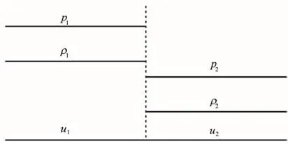
Fig. 3 Scheme of Riemann problem (Sod test)[1]

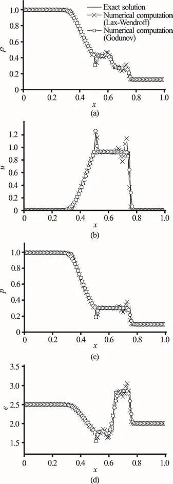
Fig. 4 Solution for the Riemann problem using the Godunov and Lax-Wendroff schemes

Figure 4 illustrates solutions to the Riemann problem using two different schemes of integration of Eqs.ously, the second-order Lax-Wendroff scheme leads to oscillations in the solution. They are evident both at the shock wave front (on the right) and at the rarefaction wave front (on the left). Unfortunately, the first-order accuracy Godunov scheme (as shown in Fig. 4) is not monotonic and also has oscillations at the rarefaction wave front. However, strong dissipative properties of the scheme can be seen in the other parts of the solution.

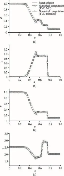
Fig. 5 Solution for the Riemann problem using the TVD scheme with minmod and MC limiters

TVD scheme with different limiters enables to decrease the oscillations in the area of strong discontinuity of parameters (as shown in Figs. 5, 6). As it turned out, the solutions to this problem obtained using different limiters do not differ from each other.However, detailed analysis of solutions shows that the superbee limiter describes the area of strong discontinuity better (two mesh points fall on the contact discontinuity) if compared for example with the minmod limiter (five mesh points fall on the contact discontinuity). In addition, the minmod limiter leads to a more monotonous distribution of hydrodynamic parameters along the whole computational domain as compared with other limiters.

Fig. 6 Solution for the Riemann problem using the TVD scheme with Van Leer and superbee limiters

Let us now consider the problem of pipe draining[8]. At the initial moment of time, the pipe with the length of 2 m is filled with air with the pressure of 1.6×105Pa and density of 2.08 kg/m3. The right end is closed, and the left one communicates with ambient air with the pressure of 105Pa and density of 1.3 kg/m3. The solution is obtained at. The parameter ζ contained in the boundary condition (2) is equal to 0.5(inflow) or -0.5 (outflow).

The experimental[8]and calculated static pressureoscillograms at the closed end of the pipe relative to the ambient pressure0p are shown in Fig. 7. The waveforms are shown over the time interval from 0-0.1s from the moment of the sudden opening of the boundary.

Obviously, the Godunov scheme leads to strong smearing of the solution. It is a property of the firstorder accuracy scheme. The Lax-Wendroff scheme leads to small oscillations at the front of the running wave. TVD scheme decreases the oscillations keeping the second-order of accuracy in computational domain.In general, the mentioned schemes are able to describe damped periodic oscillations in the pipe correctly.This result is due to taking into account the inflow and outflow energy loss in the boundary condition (2).Additionally, the velocity of disturbance propagation is well predicted (as shown in Fig. 7). The results of test calculations are in good agreement with Ref. [8].

4. A problem of steady-state resonance oscillations in semi-closed straight channel

A straight channel with the length of 1 m and the radius of 0.023 m has one open end and the other end is closed with a solid wall (as shown in Fig. 1). The“white” noise[11,15]near the open end is used as a source of noise. It is a combination of several modes of oscillations of the same amplitude distributed uniformly over a wide frequency range. One experiment with such noise source is enough to obtain amplitude-frequency responses, whereas a monochromatic noise source would require scanning across all the involved frequencies. In modelling, the periodic pressure component ()g t introduced in Eqs. (2), (5)is written as

where the summation is conducted over all harmonics i with the frequencyfrom 1 Hz to 3 000 Hz with a step of 1 Hz,=1Pa is the amplitude of the static pressure oscillations,is the random phase angle uniformly distributed over the interval from 0π to 2π.

The pressure and density of the quiescent gas in the pipe and in the ambient air are initially the same and equal to 105 Pa and 1.2 kg/m3, respectively. The drag coefficient is equal to ζ = 0 (inflow) and ζ =-1 (outflow) since the velocity profile can be considered to be uniform if the amplitude of oscilla ting velocity fluctuations is small.

Fig. 7 Static pressures at the solid boundary of the channel relative to the ambient pressures

The calculation results are compared with the experimental data. The “white” noise in the experiments is generated with the aid of a wideband speaker mounted at the distance of 2 m from the open end.Pressure oscillations are measured simultaneously at two points using acoustic equipment Bruel and Kjaer with two quarter-inch microphones 4 961. The measurements are carried out within the channel (in the middle of the closed end of the channel) and outside the channel (near the open end). Special measures are implemented in order to reduce the impact of acoustic emission from the channel on experimental results during measurements of pressure fluctuations near the open end.

The spectrum analysis shows that the amplitude of “white” noise passed to the microphone is changed in the chosen frequency range so that the frequency response of the measured signal is significantly nonuniform. Probably, the reasons for this are nonuniform frequency responses of the amplifier and the speaker systems. Therefore a transfer function ()K f is considered. It is equal to the ratio of pressure fluctuations amplitude at the closed end to the pressure fluctuations amplitude at the inlet section at the same frequency[16]. The ratio of amplitudes at the certain frequency is called an amplification factor at this frequency. The experimental transfer functionis determined as an average of five duplicate experiments. In this case the root-mean-square inlet pressure oscillations are well reproduced and differ by no more than 1% from run to run.

Solving a steady-state resonance oscillations problem for different Courant numbers, we made sure that the schemes were stable for the Courant number up to 0.7 that satisfies, furthermore, the condition of 0< 1v≤ for Godunov and Lax-Wendroff schemes[1]as well as <0.7v for TVD scheme[14]. Nevertheless,the numerical integration of Eqs. (3) using nonlinear boundary condition (2) is performed for the Courant number =0.6v atand =ΔtIn this case the number of spatial mesh nodes per wavelength is 540 (900 time steps per period of oscillation) for the first harmonic and 60(100 time steps per period of oscillation) for the fifth harmonic. Figure 8 illustrates the experimental and calculated transfer functions of pressure oscillations at the closed end in the frequency range from 1 Hz to 1 000 Hz. The calculations are performed using Godunov, Lax-Wendroff and TVD schemes. The calculation results have been obtained after reaching a steady-state oscillatory motion.

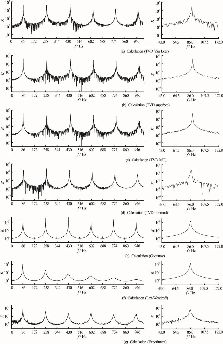
Fig. 8 Transfer functions at the closed end of the channel

Fig. 9 Static pressures at the closed end of the channel under the influence of “white” noises

Fig. 10 Static pressures at the closed end of the channel under the influence of oscillations at a single frequency

Figure 8 shows that the calculated resonance frequencies obtained using Godunov and Lax-Wendroff schemes coincide with the experimental results. One can notice the resonance at the following frequencies: 86 Hz, 258 Hz, 430 Hz, 602 Hz and 774 Hz,corresponding to the following wave resonators: 1/4,3/4, 5/4, 7/4 and 9/4. These frequencies can be calculated according to a theoretical formula, wherenf is the resonant frequency of the corresponding mode =1nN…, L is the effective length of the channelever, the Godunov scheme leads to fast decrease of the amplification factor K with the growing number of the resonance harmonic (as shown in Fig. 8).Moreover, a big difference is already observed on the sixth resonance harmonic. This deviation of the calculated transfer function is explained by the first order approximation of the time derivative in Eq. (6),which has the dissipative properties.

The results obtained using the Lax-Wendroff scheme show a trend of decrease of the amplitude of oscillations with increasing number of resonant harmonics. In general, it agrees with experimental results and theoretical concepts. But the Lax-Wendroff scheme leads to overestimated values of the transfer function at resonance frequencies. Apparently, this is mainly the result of a quasi-steady approximation for the friction

coefficient in the laminar flow ξ = 64/Re . It is known that the coefficient of hydraulic resistance ξ at high frequencies of flow oscillations increases with the growth of frequency proportional to f compared with the resistance coefficient of steady laminar flows.

Modelling of transfer function with the help of TVD scheme with MC, Van Leer and superbee limiters leads to the resonance frequency of 89 Hz (in the right part of Fig. 8). This result exceeds the experimental one by 3Hz. Minmod limiter leads to the resonance frequency of 87 Hz. Moreover, TVD scheme with limiters suggested above yields a nonuniform transfer function. A detailed analysis of the waveform of the static pressure (in the left part of Fig.9) shows that the use of limiters does not lead to a steady-state oscillatory motion. However, a cyclic static pressure (in the right part of Fig. 9) is observed over the time interval corresponding to the period of the fundamental mode of oscillation. Apparently, this behavior of solution is due to random effect of flux limiters on the result of solution. In contrast, the cyclic static pressure can be obtained using Godunov and Lax-Wendroff schemes (in the left part of Fig. 9). In this case the steady-state oscillation regime is reached 3s after the beginning of motion for Lax-Wendroff scheme and 1s for Godunov scheme.

Static pressure oscillations1p (minus the ambient pressure0p) at the closed end of the channel are shown in Fig. 10. In modelling, the discretization degree of the computational domain, the thermal properties of the working fluid and the initial properties are similar to the previous problem. In this case the gas motion in the channel is actuated by pressure fluctuations in the environment according to

Figure 10 shows that the static pressure waveforms obtained using Lax-Wendroff and TVD schemes have oscillations with different periods: 2.7 s for Lax-Wendroff scheme, 0.7 s for TVD minmod scheme, 0.3s for TVD MC, TVD superbee and TVD Van Leer schemes. As can be seen from Fig. 10,Lax-Wendroff scheme leads to a nonmonotonic achievement of steady-state periodic gas motion in the channel. This result agrees well with theoretical concepts[9,17]. In this case the stationary periodic process is established 11s after the start of movement.As noted before, the use of TVD schemes with suggested limiters does not result in stationary periodic oscillations. In addition, the amplitudes of the steady-state pressure oscillations obtained using Godunov and Lax-Wendroff schemes are almost the same and take the values of 128 Pa and 144 Pa,respectively. In contrast, Godunov scheme leads to a monotonic increase of the static pressure value at the closed end of the channel. In this case the steady-state oscillatory motion takes place 1.5 s after the start of the movement. This type of behavior is due to dissipative properties of the first-order accuracy Godunov scheme.

5. Conclusion

The problem of steady-state acoustic oscillations in a semi-closed channel actuated by external source of fluctuation has been solved in this paper. The influence of the properties of numerical schemes on the amplitude-frequency response of pressure oscillations in the straight semi-closed channel has been considered on the time scales which are many times higher than the period of oscillation. This has been shown using numerical schemes of Godunov, Lax-Wendroff and TVD. It has been found that the second-order accuracy scheme (it has been shown using the Lax-Wendroff scheme) predicts the frequency response of steady-state oscillations with sufficient degree of convergence to the experimental data. Comparing with Lax-Wendroff scheme, the use of the first-order accuracy Godunov scheme increases the prediction error of amplitude of the steady-state standing waves. TVD scheme with limiters of minmod, MC, Van Leer and superbee leads to a shift of amplitude-frequency response overestimating the value of the resonant frequency. It has been shown that the use of limiters does not lead to steady-state solution. However, a periodic pressure oscillation has been observed over a time interval corresponding to the period of the fundamental mode of oscillation.Apparently, this behavior of solution is due to random effect of flux limiters on the result of solution.

Acknowledgment

The author would like to thank Dr. Olga Dushina for technical language revision.