Anisotropy Effects and Observational Data on the Constraints of Evolution Dark Energy Models

S.A.A.Terohid and H.Hossienkhani

Department of Physics,Hamedan Branch,Islamic Azad University,Hamedan,Iran

Abstract We investigate cosmological dark energy models where the accelerated expansion of the universe is driven by a field with an anisotropic universe.The constraints on the parameters are obtained by maximum likelihood analysis using observational of 194 Type Ia supernovae(SNIa)and the most recent joint light-curve analysis(JLA)sample.In particular we reconstruct the dark energy equation of state parameter w(z)and the deceleration parameter q(z).We find that the best fit dynamical w(z)obtained from the 194 SNIa dataset does not cross the phantom divide line w(z)=−1 and remains above and close to w(z)≃−0.92 line for the whole redshift range 0≤z≤1.75 showing no evidence for phantom behavior.By applying the anisotropy effect on the ΛCDM model,the joint analysis indicates that Ωσ0=0.0163 ± 0.03,with 194 SNIa,Ωσ0= −0.0032± 0.032 with 238 the SiFTO sample of JLA and Ωσ0=0.011± 0.0117 with 1048 the SALT2 sample of Pantheon at 1σ′confidence interval.The analysis shows that by considering the anisotropy,it leads to more best fit parameters in all models with JLA SNe datasets.Furthermore,we use two statistical tests such as the usual /dof and p-test to compare two dark energy models with ΛCDM model.Finally we show that the presence of anisotropy is confirmed in mentioned models via SNIa dataset.

Key words:anisotropy effect,luminosity distance,maximum likelihood,supernova data

1 Introduction

Fairly thought of as one of the most intricate and puzzling problems in modern physics is that of the present day acceleration of the universe,[1−3](see also Refs.[4–5]for more up-to-date references).The standard explanation invokes an unknown component,usually referred to as dark energy(DE).Observational result is consistent with the picture that the universe has an unknown form of energy density,named the DE,about 70%of the total energy density.[6]A candidate for DE which seems to be both natural and consistent with observations is the cosmological constant.[6−10]However,in order to avoid theoretical problems,[7]other scenarios have been investigated.The equation of state(EoS),w,of DE,is the main parameter which determines the gravitational effect of DE on the evolution of the universe,and can be measured from observations without need to have a definite model of DE.Usually EoS parameter is assumed to be a constant with the values−1,0,−1/3 and+1 for cosmological constant(ΛCDM),dust,radiation and stif fmatter dominated universe,respectively.The simplest extension of Λ is the DE with constant w,which is the corresponding cosmological model called wCDM model.[11−12]The shortcoming of this model is that the constant w is usually viewed unphysical or unreal.However,it is a function of time or redshift[13]in general.Latest observations[14−15]from SNIa data indicate that the EoS parameter(w)is not constant.In particular,the famous examples of the former approach include scalar fields which have time varying EoS parameters such as quintessence,[16−17]K-essence,[18−19]tachyon,[20−22]phantom,[23−24]quintom,[25−26]holographic DE,[27−29]agegraphic DE[30−31]and so forth.It is worth noting that allowing w(z)to evolve with z does not seem to solve the problem.On the contrary,fitting parameterized model independent EoS parameter to the available dataset,as w(z)=w1+w2z[32−33]or w(z)=w1+w2z/(1+z)nwith n=1,2,[34−35]still points at w1< −1.However,the parametrization DE model has an evident shortcoming that it has two more additional parameters than ΛCDM,which adds enormous complexities leading to the fact that w1and w2are very difficult to be well constrained.A comprehensive comparison among the ΛCDM,the wCDM,and the w1w2CDM models with the SNIa data will be performed.

In the face of so many candidate models,it is extremely important to identify which one is the correct model by using the observational data.The measurement of the expansion rate of the universe at different redshifts is crucial to discriminate these competing candidate models.The most important way to measure the history of the cosmic expansion,is measurement of the luminocity distance relation.Since SNIa data measures the luminosity distance redshift relationship,it provides a purely kinematic record of the expansion history of the universe.In addition to investigating the effects of the observational data and their combinations on the constraints of cosmological parameters,we reconstruct the EoS parameter w(z)and the deceleration parameter q(z)by using SNIa datasets.On the other hand,the distance measurements from SNIa data depend on w(z)through double integrations,the process of double integrations smoothes out the variation of w(z).Based on the parametrization of DE model,[34−35]it was found that the ΛCDM model is inconsistent with the current data at more than 1σ′level.[36−37]Examine arbitrary parametrizations[38−41]of the expansion history H(z)and focus on maximizing the quality of fit to the SNIa dataset.These results are based on fitting a isotropic universe,together with the corresponding cosmology,to the existing astronomical data.

Moreover,recent observation data from WMAP require that the universe should achieve a slightly anisotropic special geometry in spite of the inflation.[42−45]Therefore,in an attempt to understand the observed small amount of anisotropy in the universe better,the Bianchi type models have been studied by several authors.[46−49]The Bianchi I(BI)model is sufficiently simple to allow semi-analytical calculations,and it captures the basic effect present also in more complicated anisotropic models by featuring their important common property,directiondependent expansion rates. Recently,Hossienkhani et al.[51−51]studied the effects of the anisotropy on the evolutionary behavior DE models and compare with the results of the standard Friedman-Robertson-Walker(FRW)model.Also,they have shown that the anisotropy is a nonzero value at the present time although it is approaching zero,i.e.the anisotropy will be very low after inflation.In this paper,applying anisotropy effects we shall constrain the background evolution by using SNIa data points.

This paper has the following structure.In Sec.2,we provide the exact solutions of the field equations are derived for an anisotropic BI universe and employ the SNIa data to constrain DE models.In Sec.3,we study effects of anisotropy on the constraint results of the ΛCDM,wCDM and w1w2CDM DE models and we fit the derived Hubble parameter to the SNIa dataset.In Sec.4 we briefly summarize the contents of the JLA sample and describe the light-curve fitting method and the model parameters(including those associated with the data)that are to be estimated.Conclusions and discussions on our work are given in the last section.

2 Field Equations and Supernova Data Analysis

The action for a scalar field ϕ and the Einstein-Hilbert term is described as

where g is the determinant of the metric gµν,R is the scalar curvature,V(ϕ)is the scalar potential and Smis the action of the background matter.The spatially homogeneous,anisotropic BI space-time is described by the line element

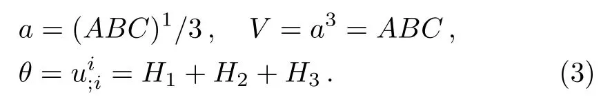
where the scale factors A(t),B(t),and C(t)are normalized as A(t0)=B(t0)=C(t0)=1 at the present(cosmic)time t0.The directional Hubble parameters are H1=˙A/A,H2=˙B/B,and H3=˙C/C,hence the mean Hubble parameter H=1/3(H1+H2+H3).The average scale factor,spatial volume,scalar expansion for the BI metric(2)are obtained respectively as

The shear scalar is defined as

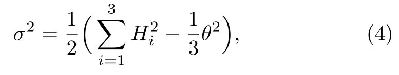
where σ2= 1/2σijσijin which σij= ui,j+(1/2)(ui;kukuj+uj;kukui)+(1/3)θ(gij+uiuj)is the shear tensor,which describes the rate of distortion of the matter flow.So,Einstein’s field equation for the BI metric is given in Eq.(2)with the help of Eqs.(3)and(4)takes the form[50−53]

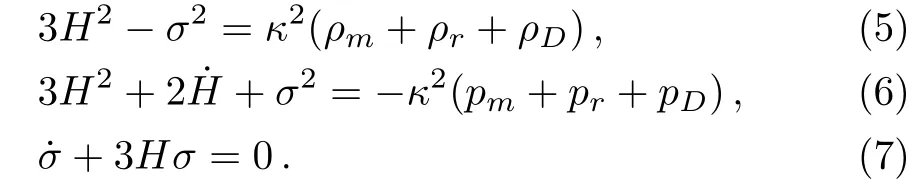
Hereafter,an overhead dot denotes differentiation with respect to cosmic time t,ρD=(1/2)˙ϕ2+V(ϕ)and pD=(1/2)˙ϕ2−V(ϕ)are the energy density and pressure of DE,respectively.It is worth noting that the density parameters are not all independent,sice evaluating Eq.(5)at the present time gives

where

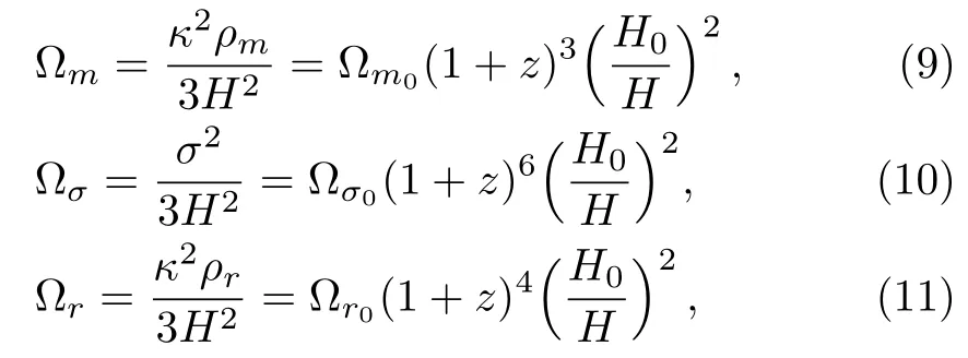
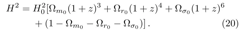
where z is the redshift,z=1/a− 1,Ωm0,Ωσ0,and Ωr0are the present value of the density parameters of matter,anisotropy and radiation respectively.Radiation density is fixed to Ωr0=2.469 × 10−5h−2(1.6903).[54]Now we described the effective EoS w(z)=p(z)/ρ(z)and the deceleration parameter q(z)=−1+(1+z)(dlnH/dz)which in general depends on the redshift z.We can express w(z)and q(z)in terms of H(z),dH/dz, Ωσ0, Ωr0,and Ωm0using the BI Eqs.(5)and(6)

In the case of generalized BI equations valid in modified gravity models,Eq.(12)can still be useful in characterizing the expansion history but it should not be interpreted as a property of an energy substance.When the anisotropy density goes to zero,i.e.σ0→ 0,and Ωσ0→ 0(i.e.spatially isotropic universe),the EoS parameter(12)is reduced to that of the Refs.[32,38–41,55–56]. It has been shown[57]that a w(z)observed to cross the line w(z)=−1 is very hard to accommodate in a consistent theory in the context of General Relativity.

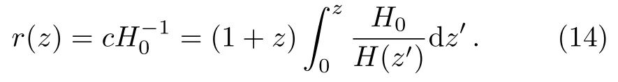
Next,we shall analyze the currently available supernova data in order to stress certain features that are inherent in such an analysis.To test reconstruction of w(z)and q(z),we choose a Hubble parameter and compute the luminosity distance dL(z)=(1+z)r(z)from the comoving distance r(z)given by

The observations directly measure the apparent magnitude m(z)of a supernova and its redshift z.The apparent magnitude m(z)is related to the luminosity distance dLof the supernova through[8,10,58−59]

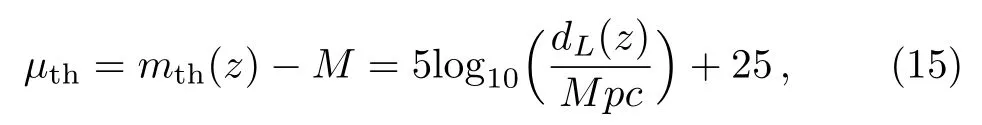
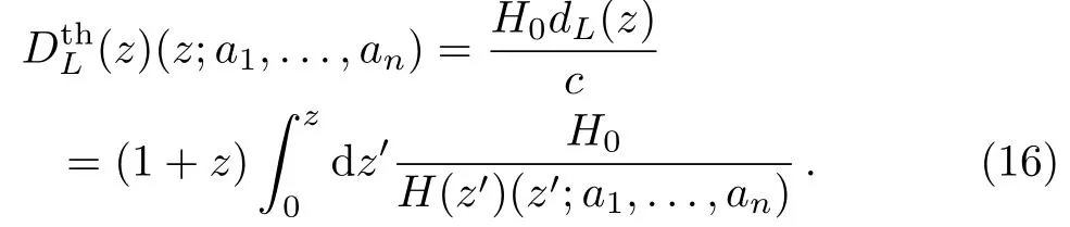
where M is the absolute magnitude(which is believed to be constant for all SNIa-this is what is called the“standard candle hypothesis”).Given a parametrization H(z;a1,...,an)depending on aiparameters we can obtain the corresponding Hubble free luminosity distance

Using the maximum likelihood technique[60]we can find the goodness of fit to the corresponding observed(i=1,...,194)coming from the SNIa dataset.[58−59]The goodness of fit corresponding to any set of parameters a1,...,anis determined by the probability distribution of a1,...,ani.e.[60]

where N is the normalization factor.Constraints on the parameter a1,...,anare obtained by the maximum likelihood method,[38]which involves the minimization of the χ2(m,a1,...,an)defined as

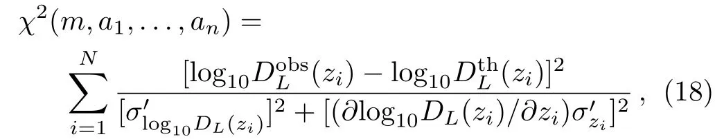
where N=194 is the number of the observed SNIa luminosity distances,are the uncertainties on the data andis the error of the SNIa distance.We also add a c−1500 km/s uncertainty in quadrature to the redshift errors given therein to account for uncertainties due to peculiar motions.[38,58−59]Note that this process is dependent on the cosmological model,and must be done for each set of cosmological parameters during the likelihood analysis.[1]The 1σ′errors on the predicted value of free parameters,a1,...,anis found by solving the following equation[60]

where a1,...,anare the values for free parameters which minimize χ2(a1,...,an).Its probability distribution is an χ2distribution for N−n degrees of freedom with 68% confidence level(C.L.)for n=1,where n is the dimensional parameter space.Also the 2σ′error with 95.4%con fidence level range which that is determined by ∆=4 for n=1 and 6.17 for n=2.

3 Maximum Likelihood Estimation and Anisotropy Effects on Various DE Models for Fit to the SNIa Dataset

This section will be devoted to introducing the SNIa datasets that we will use later on for our analysis.We will discuss the χ2estimator to be used when using SNIa as well as some useful properties of our cosmological data sample which should be taken into account in order to obtain correct results.In order to determine how effective of the anisotropy is in improving of DE models,we adopt the method of maximum likelihood estimation to our reconstruction exercise.We wish to calculate χ2as a function of the free parameters a1,...,an.Since we have SNIa distances over a wide range of redshift,we are able to marginalize over H(z)and concentrate solely on the free parameters a1,...,an.For obtaining the best-fit cosmological model from the SNIa data,one should keep in mind that the very low-redshift points might be affected by peculiar motions,so making the measurement of the cosmological redshift uncertain;hence we consider only those points which have z>0.01.We then fit 3 cosmologies to the data:a ΛCDM cosmology,a flat wCDM cosmology,and a flat w1w2CDM cosmology.

3.1 Standard Cosmology Model

Currently standard cosmological model,also known as the ΛCDM model is the simplest one with constant DE density present in the form of cosmological constant Λ and with a component with constant EoS parameter w=−1.In this case and considering anisotropy effects,the solution for H(z)can be obtained as

By fitting the ΛCDM model to the 194 SNIa data,we get197.154, Ωm0=0.276 ± 0.125,and Ωσ0=0.016 ± 0.03 at 1σ′confidence interval.The reduced χ2value is/dof=1.027.This indicates that in the ΛCDM model with considering anisotropy,it take to be the best-fit ones from SNIa data.While in the FRW model,the value of/dof is equal to 1.03.[38,61]The joint contour plots of Ωm0and Ωσ0are shown in Fig.1.

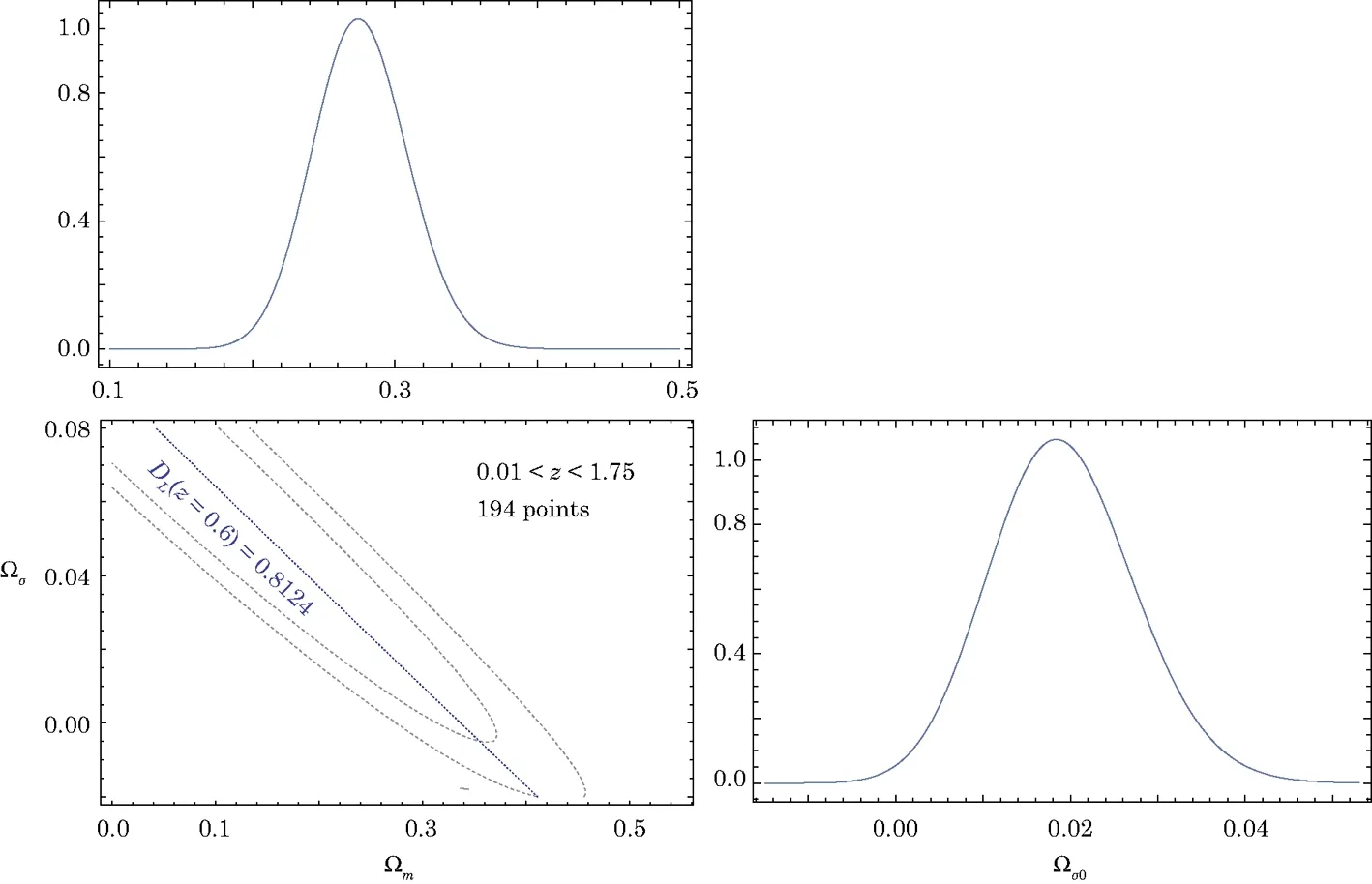
Fig.1 (Color online)The marginalized and contour plots of Ωm0and Ωσ0for the BI ΛCDM model with joint analysis base on SNIa observations.

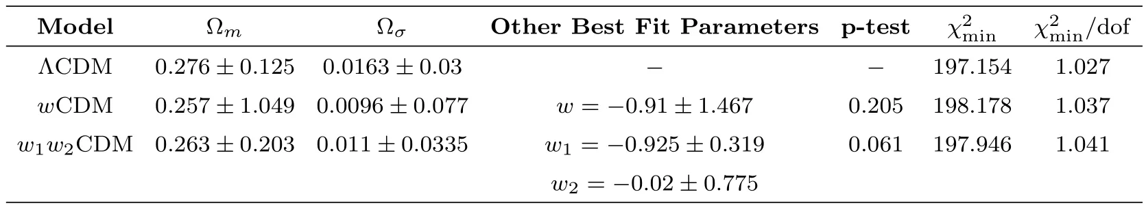
Table 1 A comparison of the DE models used in the work.

The result tells us that the flat ΛCDM model is consistent with current observational data at the 1σ′level.

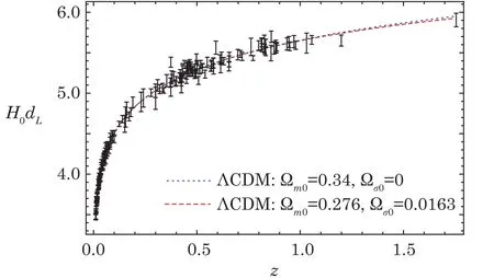
Fig.2 (Color online)A comparison the luminosity distance H0dLbetween both the isotropic and anisotropic ΛCDM models and the observational.The observational data points,shown with errorbars,are obtained from SNIa.[58−59]The blue dashed line shows the luminosity distance in the spatially flat FRW universe from Nesseris and Perivolaropoulos.[38]

The comparison the luminosity distance between both the isotropic and anisotropic ΛCDM models and the observational data from the SNIa dataset is shown in Fig.2.In order to see that the data favours models with nonzero Ωσ0,one usually plots the supernova magnitude with respect to a fiducial best-fitting mode. Table 1 lists the best-fit values of the parameters together with theand the p-teststatistic in ΛCDM model.One can see that standard rulers have considerable leverage on the joint analysis.

3.2 Dark Energy with Constant Equation of State

In this case,DE is described by a hydrodynamical energy-momentum tensor with constant EoS coefficient w=p/ρ,which leads to cosmic acceleration whenever w<−1/3.[5,17]The Hubble parameter for this generic DE component with anisotropy density Ωσ0then becomes:

For ω = −1 we recover the limiting form Eq.(20).Observational constraints on the wCDM model have been derived from many different data sets,hence it provides a useful basis for comparing the discriminative power of different data. The currently preferred values of w is given by:w= −0.98±0.12,[3]w= −1.01±0.15[62]andfrom the CMB and baryon acoustic oscillation(BAO).[63]In an anisotropic universe,SNIa alone gives w= −0.91±1.467,Ωσ0=0.0096±0.077 andΩm0=0.257±1.049(1σ′C.L.)with=198.178 anddof=1.037.This indicates that the minimization of ΛCDM model,exactly the goodness-of-fit of the wCDM model for the same data.The best fitting values and errors of the model parameters are summarized in Table 1 and Fig.3,where we also list the best fitting values of the corresponding parameters of ΛCDM model for comparison.Also,the best fit contour for w, Ωm0and Ωσ0and the marginalized probabilities of the parameter w are plotted in Fig.3.

Fig.3 (Color online)The marginalized and contour plots of Ωm0, Ωσ0and w for the BI wCDM model with joint analysis base on SNIa dataset.[58−59]

Fig.4 (Color online)Reconstructed w(z)(a)and q(z)(b)evolutions in the wCDM model using the constraint results of the current only and the current 194 SNIa data for values of Ωm0=0.257 and Ωσ0=0.0096 at the 1σ′confidence level.In both panels,the orange dashed line indicates ΛCDM model.

The evolution of w(z)with 1σ′error is shown in Fig.4(a)for the SNIa dataset.It is observed from Fig.4(a)that the present value of w(z)with 1σ′error is very close to −1.Figure 4(b)shows the evolution of the deceleration parameter q(z)with redshift z.We find that the behaviour of the deceleration parameter for the best-fit universe is quite different from that in ΛCDM cosmology.Thus,the current value of q0≃ −0.486 is significantly bigger than q0= −0.49 for ΛCDM(assuming Ωm0=0.34).Furthermore the rise of q(z)with redshift is much steeper in the case of the best-fit model,with the result that the universe begins to accelerate at a comparatively lower redshift z≃0.533(compared with z=0.57 for ΛCDM)and the matter dominated regime(q=1/2)is reached by z ∼ 1.1.

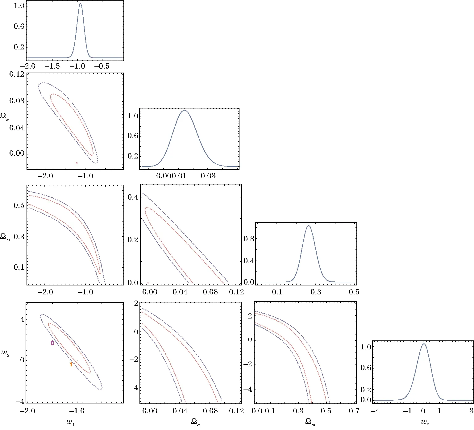
Fig.5 (Color online)Plots of marginalised likelihood functions and confidence contours on the 2D parameters space for SNIa data.The green dot correspond to ΛCDM(−1,0),the “0” point corresponds to 157 Full Gold(FG)dataset[72]and the “1” point corresponds to 115 Supernova Legacy Survey(SNLS)dataset.[73]Notice that for both the FG and SNLS dataset,the best fit occurs with Ωm0=0.3.[40]

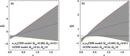
Fig.6 (Color online)Evolution of w(z)(a)and q(z)(b)parameter in the w1w2CDM model using the constraint results of the current only and the current 194 SNIa data.The thick solid line represents the best-fit,the grey contour represents 1σ′confidence level.The orange dashed line indicates ΛCDM model.

3.3 Dark Energy with Variable Equation of State

We next examine models in which DE changes with time. For a wide range of DE models,it can be shown[64−67]that,to good approximation,the DE linear EoS can be parametrized by

where w0and waare the constant.The ΛCDM model is recovered when w1=−1 and w2=0.It is noticed that the w1measures the current value of the parameter and w2gives its rate of change at the present epoch.The DE density for this case is given by

The corresponding form ofH(z) for the linear parametrization is

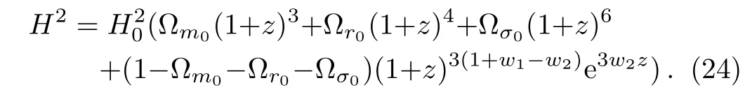
This can now be used to obtainfrom Eq.(16)and minimize the χ2obtained from the SNIa.[58−59]By using the maximum likelihood method,we obtain= 197.946;the marginalized 1σ′errors are Ωσ0=0.011± 0.0335,Ωm0=0.263± 0.203,w1=−0.925±0.319 and w2=−0.02±0.775.Comparing with the wCDM models,we find that the anisotropy effects on the linear parametrization model is a very good fit to the SNIa data.Figure 5 presents the marginalised likelihoods and confidence contours on the parameter space for 194 SNIa dataset.As it is seen that the ΛCDM model is consistent with the linear parametrization model at the 68%contour and it is almost identical with the best fit parametrization in Fig.5.Comparing with the results in Refs.[38–39,68–71],we find that the anisotropy effects improves the constraints on w1and w2significantly.

In Fig.6(a)the best fit w(z)(along with the 1σ′error region)is shown in the context of SNIa datasets for the linear parametrization.The best fit dynamical w(z)obtained from the 194 SNIa dataset does not cross the phantom divide line(PDL)w(z)=−1 and remains close to the w(z)≈ −0.92.Thus a regular single field DE Eq.(1)within the framework of GR does not seem to cross the PDL and remains in the quintessence regime.In order to alleviate this difficulty one may either introduce extra degree of freedom,[74−77]or modify the gravitational sector itself.[78−81]For model introducing in Eq.(1)if we want to source the observed expansion,we must have wϕ≃ −1,which requires a very slowlyrolling field:˙ϕ2≪V(ϕ).There has also been a lot of interest in constructing quintessence models,which can produce an EoS of the“phantom”type(wϕ< −1)[25,82]or quintom matter.[74]A quintom matter is motivated by the observational indications that the EoS of DE has to evolve below the cosmological constant boundary w=−1.Since we see that a single fluid or a single scalar field cannot give rise to quintom,so one can be introduced an additional degree of freedom to realize it.For this do,it can construct a model in terms of two scalars with one being quintessence and the other a ghost field.An alternative way to introduce an extra degree of freedom is to involve higher derivative operators in the action.This model was extensively studied in the literature in recent years(for example see Ref.[74]and references therein).The realization of quintom scenario has also been discussed within models of modified gravity,in which we can define an effective EoS to mimic the dynamical behavior of DE observed today.[78−81]

In the following we plot the evolution behavior of the deceleration parameter q(z),with the best fitting values of the Table 1 and the ΛCDM model as shown in Fig.6(b).It is clear from Fig.6(b)that the best fit values of q0and ztare in good agreement with the standard ΛCDM model(within 1σ′errors).It has been found that for the present model,q(z)shows a signature flip at the transition redshiftwhereas the transition redshift zt=0.57 for the ΛCDM model.

Till now,we have obtained the best fits for three cosmological models from 194 SNIa observations.However,the χ2statistic alone does not provide any way to compare the competing models and decide which one is preferred by the data.Therefore,we used of two criteria:(a)Luminosity distance H0dL(z);(b)Akaike Criterion(AIC)[83]and Bayesian Information Criterion(BIC).[84]

In 1998 the accelerated expansion of the universe was pointed out by the observations of SNIa.[1−2]We often use a redshift to describe the evolution of the universe.If we measure the luminosity distance observationally,we can determine the expansion rate of the universe.The comparison the luminosity distance between two flat DE models and the observational data(194 SNIa)is shown in Fig.7.This shows that the wCDM model almost coincides with the best fit parameters of the dynamical dLH0w1w2CDM models.

Fig.7 (Color online)The luminosity distance dLH0is shown as a function of cosmological redshift z for two DE models.The red and blue dashed lines show the luminosity distance wCDM and w1w2CDM models respectively.The wCDM model almost coincide with the best fit parameters of the dynamical dLH0Linear parametrizations.

Also,to assess two DE models,here we adopt the Akaike information criteria(AIC)[83]and Bayesian information criteria(BIC),[84]defined as

and BIC is given by:

where Lmaxis the highest likelihood,k is the number of free parameters and N is the number of data points used in the fits.In the Gaussian cases,= −2lnLmax.So,the difference in AIC and BIC between two models is given by∆AIC=+2∆k and∆BIC=+∆klnN respectively.In Table 2,we presentAIC,BIC,∆BIC and∆AIC for the three DE models considered in the present work.One can see that both AIC and BIC criteria support ΛCDM as the best cosmological model,in the light of current observational strong lensing data.Furthermore,it can be shown that the value of∆AIC for the observational data supports all of the models in Table 2.But for the linear model is not favored by∆BIC,though this model has slightly smaller χ2minthan the wCDM model.Finally,the deviation of the squared Hubble parameter compared to ΛCDM model determined as[38,85]

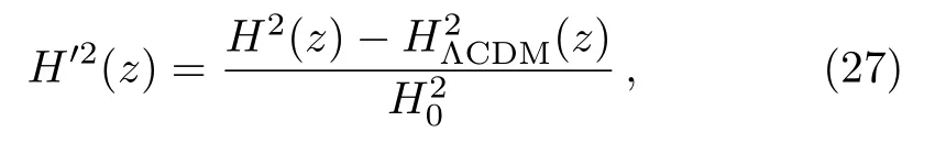
where H′2(z)isthereduced form ofH(z)and=0.7+0.3(1+z)3.In Fig.8,we plot the deviation of the squared Hubble parameter H2/from ΛCDM over redshift for the best fit.From this figure,we see that for different DE cases the reduced Hubble parameter trends seem quite similar,i.e.,the ΛCDM of BI model is,the larger the reduced Hubble expansion rate H′2(z),but in the 0 ≤ z.0.5,the curves are coincide,that is the effect of anisotropy parameter density is constant.This means that the larger the anisotropy is,the larger the exact value of the reduced Hubble expansion rate H′2(z)that we obtain.

Table 2 The minimum value of χ2,∆AIC and ∆BIC of the ΛCDM,wCDM and w1w2CDM DE models,obtained using the SNIa dataset.

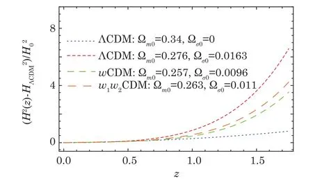
Fig.8 (Color online)The reduced Hubble parameter for some of the best and the worst fits of the cosmological models considered in Table 1.The blue dashed line denotes ΛCDM model taht the Ωm0=0.34 is assumed.[38]

4 Lightcurve and Cosmological Parameter Fitting

Here we discuss the set of previously published nearby and distant supernovae included in the analysis.Not all SN lightcurves are of sufficiently good quality to allow their use in the following cosmological analysis.To reach the goal of carrying out these improvements,we present in this paper a new SN compilation.The spectral-templatebased fit method of Ref.[86](also known as SALT)is used to fit consistently and literature lightcurve data.The most attractive feature of these events is that their absolute magnitude can be approximated by using light-curve templates to extract their “stretch” and “color” parameters,enabling them to be considered as“standardizable candles”.Guy et al.[87]presented the light curves of the SNLS SNe Ia themselves,together with a comparison of SN light curve fitting techniques,color laws,systematics and parameterizations.This catalog contains 252 highredshift SNe Ia(0.150.2.This cut,applied to both SALT2 and SiFTO samples,discards 11 SNe.There are also three SNe whose peak magnitudes could not be obtained with SiFTO due to a lack of observations in the gMand zMbands.Hence,that leaves N=238 SNLS SNe.We parameterize the SNIa light curves for distance estimation using the combined results from updated version of light curve fitter SiFTO.Finally,we constrain H(z)for the Pantheon Sample(PS)of 1048 SNe Ia,which we will supplement with the high-redshift CANDELS and CLASH SNe.The Pantheon compilation[92]included data from multiple surveys(the HarvardSmithsonian Center for Astrophysics SN surveys(CfA),the Carnegie Supernova Project(CSP),the Sloan Digital Sky Survey(SDSS),SNLS,Pan-STARRS1(PS1),the Hubble Space Telescope(HST))calibrated for a joint cosmological analysis.The Pantheon analysis employs the SALT2 light-curve fitter,[87,90]which determines an overall normalization of the SN light curve.Therefore,we perform a comparative analysis of the two most recent and reliable SNe datasets available in the work:the SiFTO sample of JLA[91](238 data points)and the SALT2 sample of Pantheon compilation[92](1048 data points).To this end,we use χ2which is defined as

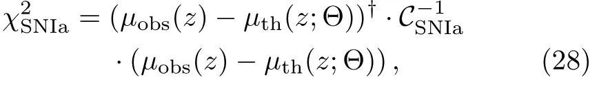
whereµthis given by Eq.(15)and correlation information of SNIa data sets is encoded in covariance matrix CSNIa(see Refs.[91-92]for more details).Following previous method,we use both SNe data to constrain three cosmological models:the ΛCDM model,the wCDM model allows a fixed,non-cosmological constant value of w,and the w1w2CDM model allows wito evolve with redshift.The constraints on these three models are presented in Table 3.Confidence contours corresponding to∆χ2=2.3(68%)and ∆χ2=6.17(95%)are shown in Figs.9 and 10.For all studies involving SNe Ia,we used likelihood functions similar to Eq.(28)with both the SiFTO sample of JLA and the SALT2 sample of Pantheon.From Table 3,it can be observed that the ΛCDM DE model has the smallest/dof.In conclusion,when our analysis is compared with that of Ref.[91],it is seen that the maximum value of the joint likelihood function in the ΛCDM of FRW model has a bigger than the maximum value of the joint likelihood function in the ΛCDM of BI model,that imply that anisotropy effects causes improves the data fitting in the ΛCDM DE model.

Table 3 Cosmological constraints for both 238 JLA SNe and 1048 Pantheon SNe samples.Values are given for three separate cosmological models:ΛCDM,wCDM and w1w2CDM DE models.

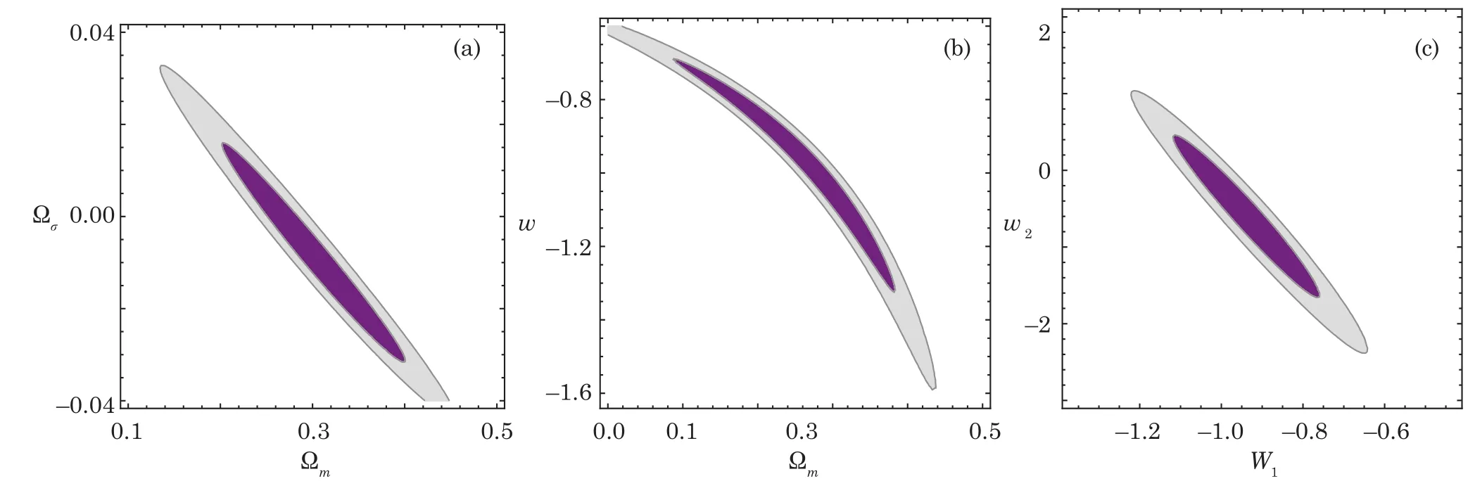
Fig.9 (Color online)Confidence contours at 68%and 95%(a)for the Ωmand Ωσ cosmological parameters for the ΛCDM model(b)for the Ωmand w cosmological parameters for the wCDM model and(c)for the w1and w2cosmological parameters for the w1w2CDM model.Constraints from JLA sample of 238 SNe Ia[91]are shown.

Fig.10 (Color online)Confidence contours at 68%and 95%(a)for the Ωmand Ωσ cosmological parameters for the ΛCDM model(b)for the Ωmand w cosmological parameters for the wCDM model and(c)for the w1and w2cosmological parameters for the w1w2CDM model.Constraints from Pantheon Sample of 1048 SNe Ia[91]are shown.

5 Conclusions

In this work we have presented some DE models when searching for an anisotropy universe using three SNIa data measurements.We have used the maximum likelihood method consisting on fitting data with the cosmological models such as the ΛCDM,wCDM and the w1w2CDM DE models.In order to place model-independent constraints on DE,we have reconstructed the EoS and deceleration parameters as a free function from current SNIa data.[58−59]Our results include an estimate of the uncertainties due to peculiar velocities=c−1500 km/s from Refs.[58–59].Since the SNIa sample data is used to estimate the luminosity distance by marginalize over free parameters in our analysis.We have solved the BI field equations and have obtained the expressions for different cosmological parameters,such as H(z),q(z),and w(z)as shown in Table 1.We have also used the minimum value of χ2,p-test,AIC,BIC information criteria and the reduced Hubble parameter and compare them with the results of the ΛCDM model.The main conclusions of our analysis comparing the three DE models in the context of the anisotropic universe may be summarized as follows:

•The second model is wCDM model and obtained the marginalized probabilities of the parameter.By fitting the 194 SNIa data to the fl at BI wCDM model,we get w= −0.91±1.467 at the 1σ′level error.The total χ2of the best fitting values of this model is=198.178 and the reduced χ2is 1.039,which is bigger than the ΛCDM model for the same datasets.On the other hand,it is shown that the wCDM model has a big value of AIC and BIC.It has been found that the evolution of q(z)in this model shows a smooth transition from a decelerated to an accelerated phase of expansion of the universe at late times.Therefore,the amount of q(z)at the current time is−0.486 and the transition redshift is z∼0.533.

•In the linear model the best fitting parameter,for SNIa data and by considering anisotropy the marginalized 1σ′errors are w1= −0.925±0.319 and w2= −0.02 ± 0.775 with=197.946 and the ΛCDM model is consistent with the current observational data at the 1σ′level.According to the rules of judgment of the AIC model selection,we conclude that recently observed data supports the w1w2CDM model as well as other popular models.To study the acceleration of the expansion of the universe,we reconstruct the deceleration parameter q(z)with a simple two parameter function and the piecewise parametrization which approximates the evolution of the universe in the redshift z.1.75.For the SNIa data,we see strong evidence that q(z)<0 in the redshiftas shown in Fig.6(b).Furthermore,it is shown that the w1w2CDM model in BI can drive the universe from a matter dominated phase to an accelerated expansion phase,behaving like matter in early times and as quintessence region,i.e.,w(z)>−1 at late times.

Although phenomenological studies of the DE component has been successful and DE models could explain the cosmic acceleration at present.There exists,however,a second approach to explain these accelerating phases,that is to modify the gravity sector itself.[78,93−95]This modification may lead to an accelerated era without invoking the DE.The f(R)theory generalises the Einstein-Hilbert action by adding additional scalar curvature invariants to the action,or by making the action a more general function of the Ricci scalar then the simple linear one that leads to Einstein’s equations.This interest was stimulated in the 1960 s,70 s and 80 s by the revelations that the quantisation of matter fields in an unquantised space-time can lead to such theories,[96]that f(R)theories of gravity can have improved renormalisation properties[97]and that they can lead to a period of late-time accelerating expansion of the universe.[98]An interesting variant on generalisations of the Einstein-Hilbert action are the f(T)theories.These models are based on the“teleparallel” equivalent of GR(TEGR),[79−81]which,instead of using the curvature defined via the Levi-Civita connection,uses the Weitzenbck connection that has no curvature but only torsion.[99]

•We also consider both the light curve fitters for our analysis.It is intended to estimate three parameters(magnitude,shape and colour)that can be subsequently linearly combined to determine the luminosity distances of the SNe Ia.Consider SN lightcurve models,we have found that,when the parameter optimization is handled via the joint likelihood function,DE models fit their individually optimized data very well.Our results for the best fit parameters of three DE models are shown in Figs.9 and 10.The best fit parameters in a ΛCDM model show interesting differences between the 194 SNIa and the JLA SNe datasets.Thus,our study shows that the anisotropy effects on the ΛCDM DE model is a very good fit to the latest JLA SNIa data.In particular,the JLA favors a flat universe much more than the 194 SNIa datasets.