
Application of Image Compression to Multiple-Shot Pictures Using Similarity Norms With Three Level Blurring
2019-06-12 01:22MohammedOmariandSouleymaneOuledJaafri
Computers Materials&Continua 2019年6期
Mohammed Omari and Souleymane Ouled Jaafri
Abstract:Image compression is a process based on reducing the redundancy of the image to be stored or transmitted in an efficient form.In this work,a new idea is proposed,where we take advantage of the redundancy that appears in a group of images to be all compressed together,instead of compressing each image by itself.In our proposed technique,a classification process is applied,where the set of the input images are classified into groups based on existing technique like L1 and L2 norms,color histograms.All images that belong to the same group are compressed based on dividing the images of the same group into sub-images of equal sizes and saving the references into a codebook.In the process of extracting the different sub-images,we used the mean squared error for comparison and three blurring methods (simple,middle and majority blurring)to increase the compression ratio.Experiments show that varying blurring values,as well as MSE thresholds,enhanced the compression results in a group of images compared to JPEG and PNG compressors.
Keywords:Image compression,simple blurring,middle blurring,majority blurring,similarity,classification,mean squared error.
1 Introduction
Images are important documents today,as it is an important part of today’s digital world.In nowadays,a huge number of companies,associations and even individuals use databases that contain a significant number of similar images.Medical clinics,has databases contain very similar X-ray images of different bones of the human body.Dentists,has databases contain very similar images for teeth and gums of different patients.The insurance company has databases contain images captured for different objects that look similar to each other’s,like similar cars.Photos are produced today more frequently than a decade ago due to the massive use of multimedia devices such as cameras,smartphones,laptops… etc.This facilitation let users enjoy taking many shots in the same place and time which produces many pictures of a high degree of similarity.However,due to the large quantity of the needed data,the storage of such data can be expensive.Thus,work on efficient image storage by compression those images have the potential to reduce storage costs.
Image compression is an application of data compression that encodes the original image with few bits.The objective of image compression is to reduce the redundancy of the image to store or to transmit in an efficient form.The compression is the process of encoding information using fewer bits or other information-bearing units than an unencoded representation.This process is useful because it helps to reduce the data redundancy to save more hardware space and transmission bandwidth.One type of data compression is known as image compression [Maini and Aggarwal (2009)].
Nowadays,a huge number of companies,associations and even individuals,use databases that contain a significant number of similar images.Medical clinics,has databases contain very similar X-ray images of different bones of the human body (Fig.1).Dentists,has databases contain very similar images for teeth and gums of different patients.

Figure 1:A set of similar X-ray images of different bones of the human body
Fashion agency,has databases contain images captured in photo shoots,each contains a sequence of pictures captured for the same persons,in the same place,with small differences in the pose.Insurance companies have databases of images captured for different objects that look similar (Fig.2).

Figure 2:Images for the same car in an accident,took by the insurance company
Even with personal devices,photos are produced today more frequently than a decade ago due to the massive use of multimedia devices such as cameras,smartphones,laptops… etc.This facilitation let users enjoy taking many shots in the same place and time resulting in many pictures with a high degree of similarity (Fig.3).
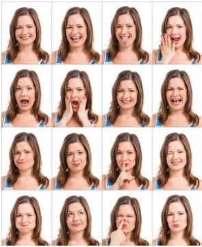
Figure 3:Set of pictures took at the same time and place for the same person with a different pose
However,due to the large quantity of the needed data,the storage of such data can be expensive.Thus,working on efficient image storage by compressing similar images has the potential to reduce storage costs.To understand this type of data compression we need first to understand the real form of the image and its structure.
Currently,thousands of algorithms and applications that perform this compression in different ways are created and developed.These applications aim to take advantage of the redundancy that appears in the image to reduce its size,using different techniques as lossy or lossless compression techniques.However,none of them are taking advantage of the redundancy that appears in a sequence of similar images to be compressed all together,in hope to reduce the storage quantity as much as possible instead of compressing each image separately.
The main objective of this work is to present a new method that aims to compress a set of images at once instead of compressing each image separately,by breaking down the entire structure of all images and then rebuild them again together with more efficient form in hope to reduce the needed storage.
There are different formats of image compressors.In fact,some formats compress some types of images better than others depending on the goal that they aim to achieve.The following table summarizes the different compression formats.

Table 1:Summary of the different formats of an image
The rest of this paper is organized as follows.In the first section,we present some basic definitions related to image compression.Our compression method and the used similarity techniques are explained in details in section three.In section four,we present the experimental results using different blurring strategies.Section five is the conclusion.
2 Lossless vs. lossy image compression
Data compression is a reduction in the number of bits needed to represent data.Compressing data can save storage capacity,speed file transfer,and decrease costs for storage hardware and network bandwidth.In this chapter,we specify the data to be an image,to define its compression,its types,its benefits,its methods and techniques,also,the evaluation methods used to evaluate the used compression technique [Bovik (2010)].
2.1 Basic definitions
Image compression is an application of data compression that attempts to reduce the image size by encoding the original image with few bits.The compression process is based on reducing the redundancy of the image to be stored or transmitted in an efficient form [Bovik (2010)].The meaning of redundancy is the duplication of data in the image.Either it may be repeating pixel across the image or pattern,which is repeated more frequently in the image [Maini and Aggarwal (2009)].In digital images,there are various types of redundancy.Image compression is achieved when one or more of these redundancies are reduced.
2.1.1 Various types of redundancy
In digital image compression,three basic data redundancies can be identified and exploited:
-Coding redundancy.
-Interpixel redundancy.
-Psycho-visual redundancy.
Data compression is achieved when one or more of these redundancies are reduced or eliminated [Pujar and Kadlaskar (2010)].
Coding redundancy
Consists of using variable length codewords selected to match the statistics of the original source,in this case,the image itself or a processed version of its pixel values.Examples of image coding schemes that explore coding redundancy are the Huffman codes [Suri and Goel (2009);Nourani and Tehranipour (2005)] and the arithmetic coding technique [Pujar and Kadlaskar (2010);Suri and Goel (2009)].
Inter pixel redundancy
Inter-Pixel Redundancy (also called spatial redundancy)is a redundancy corresponding to statistical dependencies among pixels,especially between neighboring pixels.This redundancy can be explored in several ways,one of which is by predicting a pixel value based on the values of its neighboring pixels [Pujar and Kadlaskar (2010)].
Psycho visual redundancy
It is a redundancy corresponding to different sensitivities to all image signals by human eyes.Therefore,eliminating some less relative important information in our visual processing may be acceptable [Pujar and Kadlaskar (2010)].
2.2 Types of compression
There are different techniques for compressing images.They are broadly classified into two classes called lossless and lossy compression techniques [Pujar and Kadlaskar (2010)].
2.2.1 Lossless compression
Lossless is a term used to describe an image file format that retains all the data from the initial image file [Calderbank,Daubechies,Sweldens et al.(1997)].In the lossless compression techniques,images can be compressed and restored without any loss of information.In other words,the reconstructed image from the compressed image is identical to the original one in every sense [Penrose (2001);Pujar and Kadlaskar (2010)].
Run length encoding
Run length encoding or RLE is a very simple form of image compression that performs lossless image compression [Roy and Saikia (2016)],in which runs of data are stored as a single data value and count,rather than as the original run.It is used for sequential data [Saffor,Ramli and Ng (2001)] and it is helpful for repetitive data.In this technique replaces sequences of identical value (pixel),called runs.The Run length code for a grayscale image is represented by a sequence {Vi,Ri} where Viis the intensity of the pixel and Rirefers to the number of consecutive pixels with the intensity Vi.This is most useful on data that contains many such runs,for example,simple graphic images such as icons,line drawings,and animations.It is not useful with files that don't have many runs as it could greatly increase the file size.
Entropy encoding
Entropy encoding is a lossless data compression scheme that is independent of the specific characteristics of the medium.One of the main types of entropy coding creates and assigns a unique prefix-free code for each unique symbol that occurs in the input.These entropy encoders then compress the image by replacing each fixed length input symbol with the corresponding variable length prefix-free output codeword [Nguyen,Marpe,Schwarz et al.(2011)].
Huffman encoding
Huffman coding is an entropy encoding algorithm used for lossless data compression.It was developed by Huffman.Huffman coding [Suri and Goel (2009);Nourani and Tehranipour (2005)] today is often used as a back-end to some other compression methods.The term refers to the use of a variable length code table for encoding a source symbol where the variable length code table has been derived in a particular way based on the estimated probability of occurrence for each possible value of the source symbol.The pixels in the image are treated as symbols.The symbols which occur more frequently are assigned a smaller number of bits,while the symbols that occur less frequently are assigned a relatively larger number of bits.Huffman code is a prefix code [Mathur,Loonker and Saxena (2012)].
Arithmetic coding
Arithmetic coding is a form of entropy encoding used in lossless data compression.Normally,a string of characters represented using a fixed number of bits per character,as in the ASCII code.When a string is converted to arithmetic encoding,frequently used characters will be stored with little bits and not so frequently occurring characters will be stored with more bits,resulting in fewer bits used in total.Arithmetic coding differs from other forms of entropy encoding such as Huffman coding [Pujar and Kadlaskar (2010)] in that rather than separating the input into component symbols and replacing each with a code,arithmetic coding encodes the entire message into a single number.
Lempel-Ziv-Welch coding
Lempel-Ziv-Welch (LZW)is a universal lossless data compression algorithm.LZW is a dictionary-based coding.Dictionary-based coding can be static or dynamic.In static dictionary coding,the dictionary is fixed when the encoding and decoding processes.In dynamic dictionary coding,the dictionary is updated.The algorithm is simple to implement and has the potential for very high throughput in hardware implementations [Knieser,Wolff,Papachristou et al.(2003)].It was the algorithm of the widely used UNIX file compression utility compress and is used in the GIF image format.LZW compression became the first widely used universal image compression method on computers.A large English text file can typically be compressed via LZW to about half its original size [Kaur and Verma (2012)].
2.2.2 Lossy compression
Lossy is a term meaning “with losses,” used to describe image file formats that discard data due to compression [Calderbank,Daubechies,Sweldens et al.(1997)].In lossy compression,some image information is lost,the reconstructed image from the compressed image is similar to the original one but not totally identical to it [Padmaja and Chandrasekhar (2012)].
Scalar quantization
The most common type of quantization is known as scalar quantization.Scalar quantization,typically denoted as Y=Q (x),is the process of using a quantization function Q to map a scalar input value x to a scalar output value Y.Scalar quantization can be as simple and intuitive as rounding high precision numbers to the nearest integer,or to the nearest multiple of some other unit of precision [Figueiredo (2008)].
Vector quantization
Vector quantization (VQ)is a classical quantization technique from signal processing which allows the modeling of probability density functions by the distribution of prototype vectors.It was originally used for image compression.It works by dividing a large set of points (vectors)into groups having approximately the same number of points closest to them.The density matching property of vector quantization is powerful,especially for identifying the density of large and high dimensioned data.Since data points are represented by the index of their closest centroid,commonly occurring data have low error and rare data high error.This is why VQ is suitable for lossy data compression.It can also be used for lossy data correction and density estimation [Figueiredo (2008)].
Transformation coding
In this coding scheme,transforms such as DFT (Discrete Fourier Transform)[Selesnick and Schuller (2001)] and DCT (Discrete Cosine Transform)[Khayam (2003)] are used to change the pixels in the original image into frequency domain coefficients (called transform coefficients).These coefficients have several desirable properties.One is the energy compaction property that results in most of the energy of the original data being concentrated in only a few of the significant transform coefficients.This is the basis of achieving the compression.Only those few significant coefficients are selected and the remaining ones are discarded.The selected coefficients are considered for further quantization and entropy encoding.DCT coding has been the most common approach to transform coding.It is also adopted in the JPEG image compression standard.
Fractal coding
The essential idea here is to decompose the image into segments by using standard image processing techniques such as color separation,edge detection,and spectrum and texture analysis.Then each segment is looked up in a library of fractals.The library actually contains codes called iterated function system (IFS)codes [Stenflo (1995)],which are compact sets of numbers.Using a systematic procedure,a set of codes for a given image are determined,such that when the IFS codes are applied to a suitable set of image blocks yield an image that is a very close approximation of the original.This scheme is highly effective for compressing images that have good regularity and self-similarity.
Block truncation coding
In this scheme,the image is divided into non-overlapping blocks of pixels.For each block,threshold and reconstruction values are determined.The threshold is usually the mean of the pixel values in the block.Then a bitmap of the block is derived by replacing all pixels whose values are greater than or equal (less than)to the threshold by a 1(0).Then for each segment (a group of 1 s and 0 s)in the bitmap,the reconstruction value is determined.This is the average of the values of the corresponding pixels in the original block [Delp and Mitchell (1979)].
Sub-band coding
In this scheme,the image is analyzed to produce the components containing frequencies in well-defined bands.Subsequently,quantization and coding are applied to each of the bands.The advantage of this scheme is that the quantization and coding well suited for each of the bands can be designed separately [Chen and Maher (1995)].
3 Our contribution:picture group compression
Picture group compression (PGC),is a new proposed method that takes advantage of the redundancy and the duplication not only in one image but in a set of images,to be compressed all together in hope of better compression.This method is divided into three major phases (Fig.4),each serves a specific purpose.The major phases are as follow:
-Classification phase.
-Compression phase.
-Decompression phase.

Figure 4:PGC compression
The classification phase contains a set of techniques that aim to classify the sequence of input images to groups based on specific standards.The compression phase contains many steps and processes.The first step is to blur all images to make the pixels intensity inside each image look similar in hope to improve the compression ratio of the images.Three techniques wre used in blurring:simple blurring,middle blurring,and majority blurring.The next step is to create a codebook where we divide the entire set of images to sub-images based on a given size,and then extract the distinct sub-images only.Then,the distinct sub-images are all assembled to form the codebook.To extract the distinct subimages,two methods are used:similar blocks,and MSE (mean squared error).Afterwards,index files are created where each image is replaced by its sub-images indices based on its position in the codebook.At the end o,both the codebook and index files are combined together and form the compressed version of the input images.The decompression phase consists of replacing the indices with their corresponding subimages inside the codebook.Preliminary results of this work can be found in Omari et al.[Omari,Jaafri and Karour (2016)].
3.1 Classification phase
The classification is the process of gathering the entire images based on specific criteria,forming a set of groups of similar images.Each group shares a bunch of characteristics that depend on the chosen technique of classification.In fact,there are considerable numbers of similarity based classification technique.
3.1.1 L1and L2norms
L1Norm,Manhattan norm,or the sum of absolute intensity differences [Schmidt (2005)] is one of the oldest similarity measures used to compare images.Given two images X and Y where:
X={ xi∶i=1,2,…n}
y={ yi∶i=1,2,…n}
xiand yirepresenting intensities of the corresponding pixel in the two images X and Y in raster scan order,the L1Norm between the images [Bishop (2006)] is defined by:

L1Norm is position based,which compare the images X and Y pixel by pixel.So,if the image Y is identical to the image X in the content,but,there are is a small shift,this measure can produce matching results that refer to no similar images.The same unwanted result when it comes to identical images taken under different lighting condition [Yin,Esser and Xin (2014)].
Square L2Norm,square Euclidean distance [Duda,Hart and Stork (2012)],or sum of squared intensity differences of corresponding pixels in sequences X={ xi∶i=1,2,…n} and y={ yi∶i=1,2,…n} is defined by:
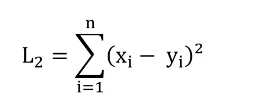
Compared to L1Norm,square L2Norm emphasizes larger intensity differences between X and Y,also it is more sensitive to the magnitude of intensity difference between images,and therefore,it will produce poorer results when used in the matching of images taken under different lighting conditions [Yin,Esser and Xin (2014)].
3.1.2 Color histograms
The color histogram is a vector where each entry stores the number of pixels of a given color in the image.Color histograms are frequently used to compare images and widely used for content-based image retrieval [Sharma,Rawat and Singh (2011);Roy and Mukherjee (2013)].Their popularity stems from several factors:
-Color histograms are computationally trivial to compute.
-Small changes in camera viewpoint tend not to effect color histograms.
-Different objects often have distinctive color histograms.
-Do not relate spatial information with the pixels of a given color.
-Color histograms are robust against occlusion.
-Largely invariant to the rotation and translation of objects in the image.
A color histogram H is a vector(h1,h2,…,hn),in which each bucket hjcontains the number of pixels of color j in the image.
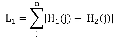
For a given image X,the color histogram H is a compact summary of the image.A database of images can be queried to find the most similar image to X.Typically color histograms are compared using the sum of squared differences (L2-distance)or the sum of absolute value of differences (L1-distance).
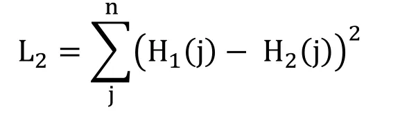
Given two images X and X’ with the color histogram H1and H2respectively.The L1-distance defined as:
And the L2-distance defined as:
3.1.3 Color appearance
The Color Appearance is a very simple proposed technique of similarity measures which is based on comparing the appearance of the unique color in both images rather than comparing the redundancy of the color.In other words,unlike the histogram technique,the redundancy of color is not important,only the presence of color in both images raise the value of similarity.
Given two images X and Y,Ixand Iyrepresenting the sequences of unique intensities values where:
Ix={ xi∶i=1,2,…n}
Iy={ yi∶i=1,2,…m}
Let T be the number of the unique intensities values that appear in both sequences Ixand
Iy.The Color Appearance can be defined as:
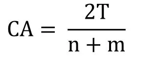
CA takes values between 0 and 1,where if the CA value is equal to 0 means the two images X and Y are totally deferent.Whereas,if the CA value is equal to 1 means that the two images are totally similar.
3.1.4 Pearson correlation coefficient
The Pearson Correlation Coefficient [Omhover,Detyniecki and Bouchon-Meunier (2004)] between two given sequences X and Y where X={ xi∶i=1,2,…n} and y={ yi∶i=1,2,…n} can be defined as:

3.1.5 Color coherence vectors
Color coherence is the degree to which pixels of that color are members of large similarly colored regions.It is referred to these significant regions as coherent regions,and observe that they are of significant importance in characterizing images.The coherence measure classifies pixels as either coherent or incoherent.Coherent pixels are a part of some sizable contiguous region,while incoherent pixels are not.A Color Coherence Vector (CCV)represents this classification for each color in the image [Roy and Mukherjee (2013);Ravani,Mirali and Baniasadi (2010)].This notion of coherence allows us to make fine distinctions that cannot be made with simple color histograms.
The initial stage in computing a CCV is similar to the computation of a color histogram,which consists of blurring the image slightly by replacing pixel values with the average value in a small local neighborhood,then discretize the color space,such that there are only n distinct colors in the image.
The next step is to classify the pixels within a given color bucket as either coherent or incoherent.A coherent pixel is part of a large group of pixels of the same color,while an incoherent pixel is not.We determine the pixel groups by computing connected components.A connected component C is a maximal set of pixels such that for any two pixels p,p′∈C,there is a path in C between p and p’.Formally,a path in C is a sequence of pixels p=p1,p2,…,pn=p′ such that each pixel piis in C and any two sequential pixels pi,pi+1are adjacent to each other.We consider two pixels to be adjacent if one pixel is among the eight closest neighbors of the other,in other words,diagonal neighbors are included.
After classifying the pixels,the next process is computing the connected components,which can be applied in a single pass over the image.In the end,each pixel will belong to exactly one connected component.We classify pixels as either coherent or incoherent depending on the number of pixels of its connected component.A pixel is coherent if the size of its connected component exceeds a fixed value τ,otherwise,the pixel is incoherent.
3.1.6 Comparing CCV's
Consider two images X and X’,and their CCV’s G and G’ respectively,and let the number of coherent pixels in color bucket j be αjfor X,and α′jfor X’.Similarly,let the number of incoherent pixels be βjand β′jfor the images X and X’ respectively.We can define G and G’ using the following expression:
G=((α1,β1),…,(αn,βn))
G′=((α′1,β′1),…,(αn′,β′n))
Comparing the images X and X’ can be done based on the following term:

3.1.7 Normalization CCV's
The final step is the normalization step.Without normalization,the distance between the coherence pairs (0,1)and (0,100)is as large as the distance between (9000,9001)and (9000,9100).The normalized difference between G and G’ can be calculated using the following term:
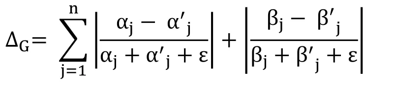
The denominators normalize these differences with respect to the total number of pixels.The factor of ε is a very small number used to avoid division by zero when α's or β's are null.
3.1.8 Sub-image based similarity
Calculating the similarity between two images using the color histogram is based on calculating and comparing the number of pixels of a given color in the images.Instead,this proposed technique of Sub-image Based Similarity is based on comparing subimages of given fixed size.In this technique,we need to divide each image into subimages,then compare sub-images based on the similarity threshold.
Given two images X and Y,we extract two sets of sub-images (Sxand Syrespectively)that represent the sequences of unique sub-images:
Sx={ xi∶i=1,2,…n}
Sy={ yi∶i=1,2,…m}
Let T be the number of the unique sub-images that’s appear in both sequences Sxand Sy.
The Sub-image Based Similarity can be defined as:
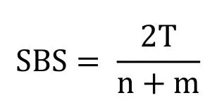
The SBS value is always between 0 and 1;SBS=0 means that the two images X and Y are totally deferent,whereas,SBS=1 means that the two images are totally similar but not necessarily identical.
So given a set of images (or pictures),we need to perform classification into groups based on similarity,then apply the compression to each group in order to achieve better results in terms of compression ratio and decompressed image quality.
3.2 Compression phase
After the process of classification,which each similar set of images are gathered based on specific criteria’s that we already mentioned.Now,we move on to the compression phase,which consists of breaking down the entire structure of the similar group of images and rebuilt them again with more organized form,in order to reduce the size of the entire images.In this phase,a sequence of steps needs to be applied over those similar images,to perform the process of rebuilding the structure of images.
3.2.1 Blurring
In the process of taking images using a camera,the small budge of the camera causes us unnoticeable changes to the human eye.Yet,when it comes to lighting,a small change is may affect the entire image.For instance,Fig.5 shows two similar images X and Y that were taken in the same lighting condition and in the same position with shooting time difference of 3 seconds.
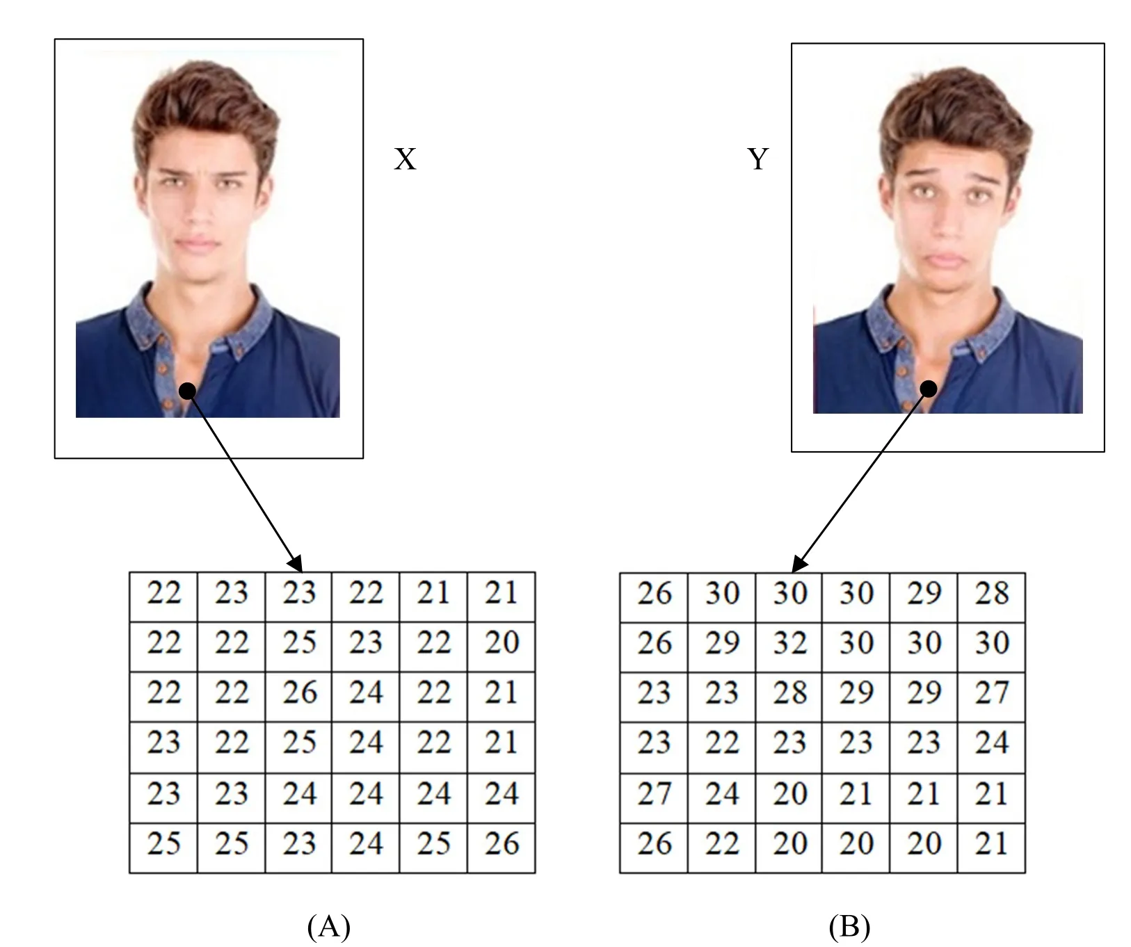
Figure 5:Extracting same-position sub-images from two similar images
When extracting two sub-images A and B from X and Y respectively A=X(370:375,175:180),B=Y(370:375,175:180)),we noticed that the sub-images might be considered not similar if a threshold value is not respected.
The blurring techniques came to solve these kinds of similarity problems.In the blurring technique,the input images are slightly blurred,by discretize the color space such that there are only n distinct colors in the images [Wang,Huang,Yan et al.(2009);Queiroz,Ren,Shapira et al.(2013)].The blurring technique requires defining the blurring value,which used to split the intensity values in the image to intervals,each value belongs to the interval is replaced by one value based on the used blurring technique.In our experiments,we used the simple blurring,the middle blurring,and the majority blurring.The n distinct colors value depends on the chosen blurring technique and the blurring value.
Simple blurring technique
In the simple blurring,the pixel intensity values of the image are split to intervals based on the blurring value (where the blurring value is the length of the interval).All values that belong to an interval are replaced by the smallest value in the same interval.Fig.6 shows the process of blurring using a simple blurring technique.
Given a blurring of 5,both image intensity values of A and B are split into intervals of length equal to 5.All values that belong to an interval are replaced by the smallest value of the same interval as is shown in Fig.7.

Figure 7:The images A' and B' representing the images X' and Y' after blurring using simple blurring technique
After blurring and discretizing the color space,the resulted image A' contains only two distinct intensity values instead of six,while B' contained three values.Furthermore,the two images carried very much similar data after the blurring process,which will positively affect the process of compression.
Middle blurring technique
Middle blurring is similar to the simple blurring,but the values that belong to an interval are replaced by the middle value rather than the smallest value.Given a blurring value also equal to 5,the blurring of images A and B is shown in Fig.8:
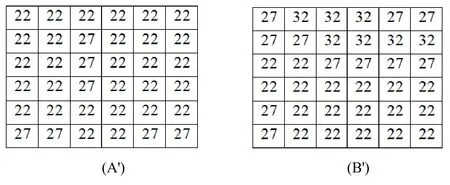
Figure 8:The images A' and B' representing the images X and Y after blurring using the middle blurring technique
As in simple blurring,the resulted two images contained two and three intensity values respectively,which bring more similarity.However,the middle blurring showed that the resulting intensity values are closer to the original images.
Majority blurring technique
In the majority blurring technique,all values that belong to an interval are replaced by a new value that belongs to the same interval and it is the most frequent value in the whole image.In this case,the modification in the image is less than that of simple and middle blurring techniques.To extract the most frequent values in the entire image,the histogram technique is used as follows:We extract all unique intensity values in the image,and then we calculate their redundancy.The following example shows the process of blurring using a majority blurring technique.

Table 2:The redundancy of each unique intensity value
Using Tab.2,we can apply the majority blurring technique on both images A and B as it is shown in Fig.9.

Figure 9:The images A' and B' representing the images A and B after blurring using the majority blurring technique
As in simple and middle blurring,the resulted two images contained two and three intensity values respectively,which bring more similarity.However,the majority of blurring showed lesser modifications.
4 Experiments and results
The PGC uses many parameters to perform compression:The blurring value (0 to 6),the sub-image size (3,4,5,and 6),the MSE value (0 to 30),and the number of images in a group.As shown in Fig.10,we chose a set of similar images from Alamy database (www.alamy.com).For comparison purposes,we used JPEG and PNG compressions.

Figure 10:Test images
4.1 Results using simple blurring
Fig.11 shows that the compression ratio is directly proportional to the blurring values when PGC compression is used.However,the PSNR decreased up to half when reaching a blurring value of 30.In addition,the compression ratio of PGC was always higher than PNG and exceeds that of JPEG when a blurring value of 25 is reached.We noticed in these experiments that the chosen sub-image size affected much neither the compression ratio nor the PSNR.
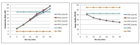
Figure 11:Compression results using simple blurring
4.2 Results using middle blurring
The obtained results using middle blurring were almost identical to simple blurring.Fig.12 shows that the compression ratio is directly proportional to the blurring values when PGC compression is used.However,the PSNR also decreased up to half when reaching a blurring value of 30.In addition,the compression ratio of PGC was always higher than PNG and exceeds that of JPEG when a blurring value of 25 is reached.We noticed,as in simple blurring,that the chosen sub-image size affected much neither the compression ratio nor the PSNR.On the other hand,the PSNR was enhanced compared to simple blurring.

Figure 12:Compression results using middle blurring
4.3 Results using majority blurring
The obtained results using majority blurring were not enhanced compared to simple and middle blurring.Fig.13 shows that the compression ratio is directly proportional to the blurring values when PGC compression is used.However,the PSNR also decreased up to half when reaching a blurring value of 30.In addition,the compression ratio of PGC was always higher than PNG and exceeds that of JPEG when a blurring value of 22 is reached.We noticed,as in simple and middle blurring,that the chosen sub-image size affected much neither the compression ratio nor the PSNR.On the other hand,the PSNR was decreased compared to middle blurring.

Figure 13:Compression results using majority blurring
4.4 Results using mean squared error with no blurring
In this sequence of experiments,the MSE method is used to compress the image with no blurring.Both MSE and the sub-image sizes are varied.

Figure 14:Compression results using MSE without blurring
As we can notice from Fig.14,a serious variation appear all over the CR and the PSNR each time we change the sub-image size and the MSE value.The CR of PGC increased up using sub-image length equal to 6 and MSE value also equal to 6.
In fact,the higher the MSE value,the higher the number of group blocks that are replaced by a single block which increases the CR,and vice versa.Also,when the sub-image size gets higher,the number of pixels the number of blocks inside an image gets lower,which increases the CR.
4.5 Results using mean squared error with blurring
In this set of experiments,the MSE method is used to compress the image using middle blurring technique with blurring value equal to 5.
We can notice in Fig.15 the huge changes in the CR using PGC with the MSE method,where the CR is increased by raising both MSE value and sub-images size.Adding the third factor which is the image blurring helped in raising the CR with acceptable and sometimes good PSNR.
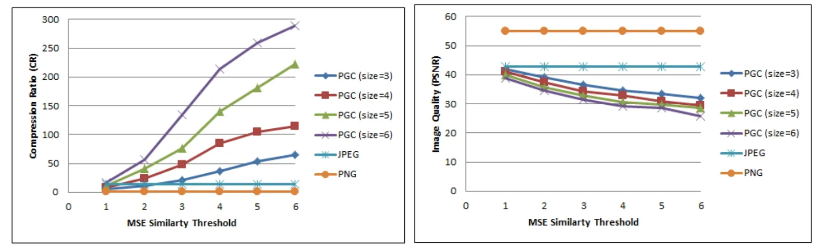
Figure 15:Compression results using MSE with blurring
5 Conclusion and future work
Image compression techniques are based on reducing the redundancy and the duplications that appears in the image to store or to transmit in an efficient form.In this paper,we introduced with the idea of picture group compression (PGC),where a set of images and pictures are compressed all together after classification into a group based on similarity.The compression process is applied over one group at a time in hope to reach higher compression results.In our method,we used three blurring techniques in order to increase redundancy and thus compression ratio.Also,a mean squared error value was varied to detect similarity and enhance compression.The results of applying both blurring and mean squared error techniques were better compared to applying each technique solely.As a future work,we aim to develop a better mechanism for extracting unique blocks without negatively affecting the PSNR and extending our work to videos.
Conflicts of Interest:The authors declare that there is no conflict of interest regarding the publication of this article.
 Computers Materials&Continua2019年6期
- Computers Materials&Continua的其它文章
- Development of Cloud Based Air Pollution Information System Using Visualization
- A Learning Based Brain Tumor Detection System
- Shape,Color and Texture Based CBIR System Using Fuzzy Logic Classifier
- LRV:A Tool for Academic Text Visualization to Support the Literature Review Process
- On Harmonic and Ev-Degree Molecular Topological Properties of DOX,RTOX and DSL Networks
- A Reliable Stochastic Numerical Analysis for Typhoid Fever Incorporating With Protection Against Infection