
Relation Extraction for Massive News Texts
2019-07-18 01:59LiboYinXiangMengJianxunLiandJianguoSun
Computers Materials&Continua 2019年7期
Libo Yin, Xiang Meng, Jianxun Li and Jianguo Sun,
Abstract: With the development of information technology including Internet technologies, the amount of textual information that people need to process daily is increasing.In order to automatically obtain valuable and user-informed information from massive amounts of textual data, many researchers have conducted in-depth research in the area of entity relation extraction.Based on the existing research of word vector and the method of entity relation extraction, this paper designs and implements an method based on support vector machine (SVM) for extracting English entity relationships from massive news texts.The method converts sentences in natural language into a form of numerical matrix that can be understood and processed by computers through word embedding and position embedding.Then the key features are extracted, and feature vectors are constructed and sent to the SVM classifiers for relation classification.In the process of feature extraction, we had two different models to finish the job, one by Principal Component Analysis (PCA) and the other by Convolutional Neural Networks (CNN).We designed experiments to evaluate the algorithm.
Keywords: Entity relation extraction, relation classification, massive news texts.
1 Introduction
Relation extraction is the task of predicting attributes and relations for entities in a sentence [Mooney and Bunescu (2005)].For example, given a sentence “Liu works in Alibaba”, the user may want to extract the semantic relationship between Liu and Alibaba.Relation extraction is the key component for building relation knowledge graphs, and it is of crucial
significance to natural language processing applications such as structured search, sentiment analysis, question answering, and summarization [Liu, Shen, Wang et al.(2005)].
Relation extraction problem can be seen as a classification problem for data containing relational information.Initially, people used rule-based approaches to solve this problem, but the implementation of this kind of approaches requires a lot of labor from experts and linguists in specific fields [Qu, Ren, Zhang et al.(2017)].In order to overcome the shortcomings of the rule-based approaches, people began to use machine learning methods to solve this problem, greatly reducing the cost of relation extraction.The machine learning methods at that time need to construct the training data in the form of feature vectors, and then use the machine learning algorithm to construct the classifiers to classify the relationship types.Therefore, this kind of methods is also called the featurebased methods [Lin, Shen, Liu et al.(2016)].Later, Kernel-based methods were introduced, which were originally introduced in support vector machine and later extended too many other algorithms.Compared with the feature-based methods, the Kernel-based methods do not use the feature vectors as input, but directly use the original string as the operation object of the model, and solve the Kernel (Similarity) function between the two target objects [Gormley, Mo and Dredze (2015)].But the fatal flaw of this type of method is that training and prediction are extremely slow and not suitable for the processing of large amounts of textual data.Besides, among all the machine learning approaches for supervision, the CNN model achieved state-of-the-art performance in the field of natural language processing.
In this paper, we investigate the effect of PCA and shallow CNN for the extraction of a large number of news texts.We convert natural language texts that do not have structured information into numerical representations, then extract the text features on this basis.According to the extracted features, the relationship types of the existing pairs of objects included in the texts are classified for the extraction of the English entity relation.In this process, the process of training the model, testing the model, and adjusting the parameters needs to be repeated to achieve the best extraction effect.
The contributions of this paper can be summarized as follows:
● We avoid the complex process of traditional feature extraction by CNN and PCA.
● We avoid the vanishing gradient problem caused by deep CNN by using shallow CNN and support vector machine (SVM).
2 Structure
In this section, we describe two models of SVM for relation extraction.One makes use of PCA to get feature vectors while the other makes use of CNN.
2.1 Vector representation
Let xibe the i-th word in the sentence and e1, e2 be the two corresponding entities.Each word will access two embedding look-up tables to get the word embedding WFiand the position embedding PFi.Then, we concatenate the two embeddings and denote each word as a vector of vi=[WFi,PFi].
2.1.1 Word embeddings
Each representation vicorresponding to xiis a real-valued vector.All of the vectors are encoded in an embeddings matrix Vw∈ℝdw×|V|where V is a fixed-sized vocabulary.
2.1.2 Position embeddings
In relation classification, we focus on finding a relation for entity pairs.Following Zeng et al.[Zeng, Liu, Lai et al.(2014)], a PF is the combination of the relative distances of the current word to the first entity e1 and the second entity e2.For instance, in the sentence “Steve_Jobs is the founder of Apple.” the relative distances from founder to e1 (Steve_Jobs) and e2 are 3 and -2, respectively.We then transform the relative distances into real-valued vectors by looking up one randomly initialized position embedding matrices Vp∈ℝdp×‖P‖where P is fixed-sized distance set.It should be noted that if a word is too far from entities, it may be not related to the relation.Therefore, we choose maximum value emaxand minimum value eminfor the relative distance.
In the example shown in Fig.1 it is assumed that dwis 4 and dpis 1.There are two position embeddings: one for e1, the other for e2.Finally, we concatenate the word embeddings and position embeddings of all words and denote a sentence of length n (padded where necessary) as a vector

Where ⊕ is the concatenation operator and vi∈ℝd(d =dw+dp×2).
2.2 Extracting feature vectors by PCA
Principal Component Analysis (PCA) is a multivariate statistical analysis method that studies how to reflect most of its information through a few linear combinations of original data.
Principal component analysis converts multiple variables into several integrated variables by reducing the dimensionality of the original analytical data, while losing less information.Usually, the integrated variable obtained by the conversion is called the principal component.Among them, each principal component represents a linear combination of the original variables, and the variables in this linear combination have no correlation, so the principal component has better performance than the original variables.In this way, when studying complex problems, only a few principal components can be considered, and complex problems can be simplified without losing too much information, which improves the efficiency of analyzing complex problems.
The principle of principal component analysis is to project the original sample data into a new space.If the sample data is represented by a matrix, it is equivalent to mapping a set of matrices to another coordinate system.However, in the new coordinate system, it means that the original sample does not need so many variables, and only the eigenvalue of the largest linear independent combination of the original sample corresponds to the coordinates of the space.
Therefore, the PCA replaces the original n feature variables with a smaller number of k feature variables, and projects the n-dimensional features into the k-dimensional coordinate system.The k variables are linear combinations of the original variables, the linear combination samples have the largest variance, and the k characteristic variables are uncorrelated.PCA reduces the n-dimensional data variable to k-dimensional and can be used for data compression, but PCA must ensure that the information loss of the data is as small as possible after the dimension is reduced.In other words, the PCA needs to find a projection direction for the original data space to maximize the data variance information after projection, which helps to retain as much valuable information as possible.
As shown in Fig.1, after flattening the original input matrix, the PCA algorithm can compress the n×ℎ vector into a smaller size feature vector.
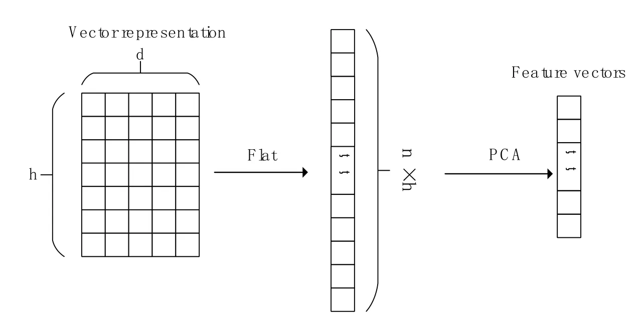
Figure 1: The process of PCA for extracting features
2.3 Extracting feature vectors by CNN
CNN, as a common variant of traditional artificial neural networks, is an important feedforward neural network that has been successfully applied in the field of image recognition and speech processing.The main features of CNN are locally connecting weights sharing, and pooling.Locally connecting is inspired by the working mechanisms of the biological visual system.The global information acquired by human visual nerves is obtained through the combination of local information.This is a bottom-up feature extraction method.The meaning of weights sharing is that when using CNN for local connections, different parts of the data share the same weights.On the one hand, this approach conforms to the objective process of human cognition, and on the other hand, it reduces a large number of network parameters and reduces the complexity of the model.The meaning of the pooling operation is to discard the redundant and non-critical information received during the identification process without destroying the overall characteristics of the target object, further reducing the calculation.
Fig.2 describes the architecture of our model with CNN to extract features.
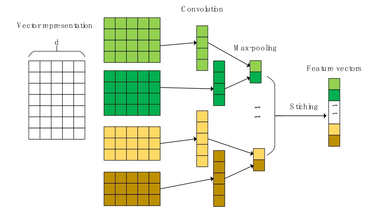
Figure 2: The architecture of CNN used for extracting features
2.3.1 Convolution
Let vi:i+jrefer to the concatenation of words vi, vi+1, …, vi+j.A convolution operation involves a filter w ∈ℝℎd, which is applied to a window of ℎ words to produce a new feature.A feature ciis generated from a window of word vi:i+ℎ-1by

Here b ∈R is a bias term and f is a non-linear function.This filter is applied to each possible window of words from v1to vnto produce feature c=[c1,c2, …,cn-ℎ+1] with c ∈ℝs(s=n(s=n-ℎ+1).
2.3.2 Global pooling on feature maps
In the output of the convolution operation, it contains key information and redundant information.Through the pooling operation, redundant information in the data can be discarded without destroying the main features of the data.
In our algorithm, we have designed a global maximum pooling strategy on the feature maps.For the feature maps obtained by the convolution operation, we use the filters with the same size of the feature maps for maximum pooling operation on each feature map, which makes each feature map finally generate a single feature value.By splicing all the eigenvalues, we can get the feature vectors we need [Zheng, Lu, Bao et al.(2017)].We apply a max-pooling operation on a feature map and take the maximum valuemax{c}.We have described the process by which one feature is extracted from one filter.We take all features into one high level extracted feature vector z=(note that here we have m filters).
2.4 SVM for relation classification
The SVM method is a traditional machine learning algorithm that plays an important role in the field of artificial intelligence.It has excellent performance in many classification tasks.Therefore, it is widely used in many tasks in the industry.Compared with naive Bayes algorithm, k-nearest neighbors algorithm and decision tree algorithm, SVM method not only has a better classification effect but also has stronger robustness, better generalization ability and better high-dimensional data processing characteristics.
The main idea of SVM can be obtained from Eq.(3).The vector x represents the input sample data.Determine a hyperplane in space, w=[w1,w2,w3,…,wd] is the normal vector of the hyperplane, and b is the offset of the hyperplane.For any input x, the hyperplane equation can give a positive or negative label yias a result of the classification.

Fig.3 shows the SVM classification effect in two-dimensional space.For inputs in highdimensional space, the SVM will find high-dimensional hyperplanes that have the same classification effect as the lines in Fig.3.When the input data cannot be classified in the current dimension, we can use the kernel method to map the data to a higher dimensional space for classification.The use of the kernel method makes SVM more powerful and can solve more complex classification problems in high-dimensional space, which is one of the reasons why SVM continues to be hot.
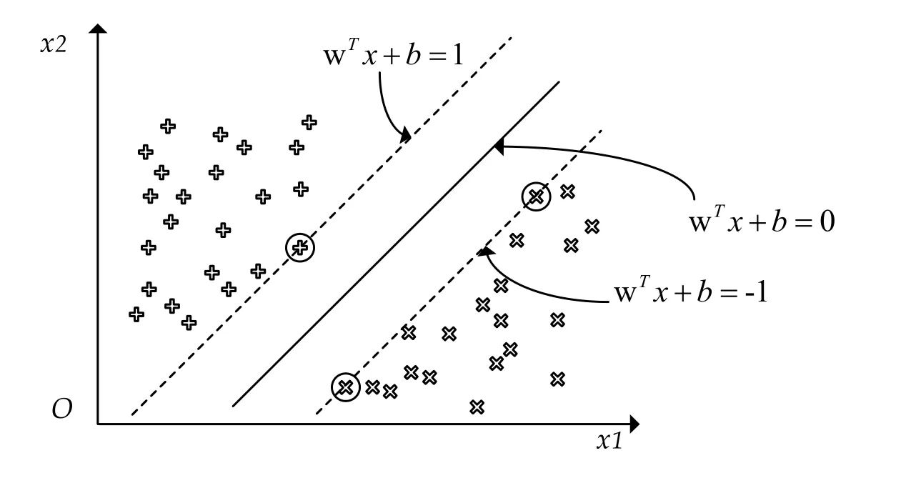
Figure 3: SVM classification in two-dimensional space
In this paper, the corpus is divided into a training set and a testing set.The feature vectors are obtained after that the texts are processed as input through word embedding, position embedding and feature extraction.Besides, the feature vectors from the training set are used to train the SVM classifiers constructed in a one-versus-rest or one-versus-one manner.The classifiers have the ability to perform multi-classification of relationships, that is, it is determined whether the type of relationship between the pair of entities in the current sample matches one of the predefined relationships.After that, the feature vectors from the testing set are sent to the trained classifiers to finish the relation extraction of the testing set.
Fig.4 shows the main process of our relation extraction algorithm.

Figure 4: The steps for relation extraction with SVM
3 Experiments
3.1 Experimental settings
In this paper, we use the word embeddings released by Lin et al.[Lin, Shen, Liu et al.(2016)] which are trained on the NYT-Free base corpus [Riedel, Yao and Mccallum (2010)].We fine tune our model using validation on the training data.The word embedding is of size 50.The input text is padded to a fixed size of 100.
3.1.1 Experimental Settings for PCA-SVM
In this lab, we used the open source Scikit-learn machine learning package to implement the PCA and SVM we needed.We transform the input matrix into a one-dimensional vector and then use PCA to extract features in a dimensionally reduced manner.In this process, different dimensionality reduction ratios produce feature vectors of different sizes.
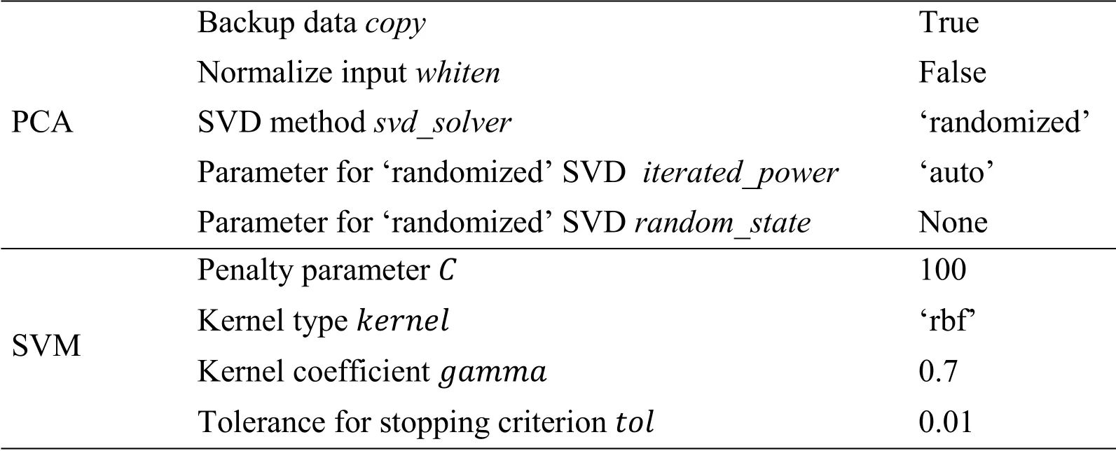
Table 1: Parameter settings for PCA-SVM
3.1.2 Experimental settings for CNN-SVM
Training is performed with Tensorflow adam optimizer, using a mini-batch of size 64, an initial learning rate of 0.001.We initialize our convolutional layers following Glorot et al.[Glorot and Bengio (2010)].The implementation is done using Tensorflow 1.3.All experiments are performed on a single NVIDIA GeForce GTX 1080 GPU.
After extracting feature vectors from the embedded matrix, we need to train our SVM model to process the feature vectors.We make use of the Scikit-learn package for machine learning to implement our SVM.
In Tab.2 we show all the parameters used in the experiments.
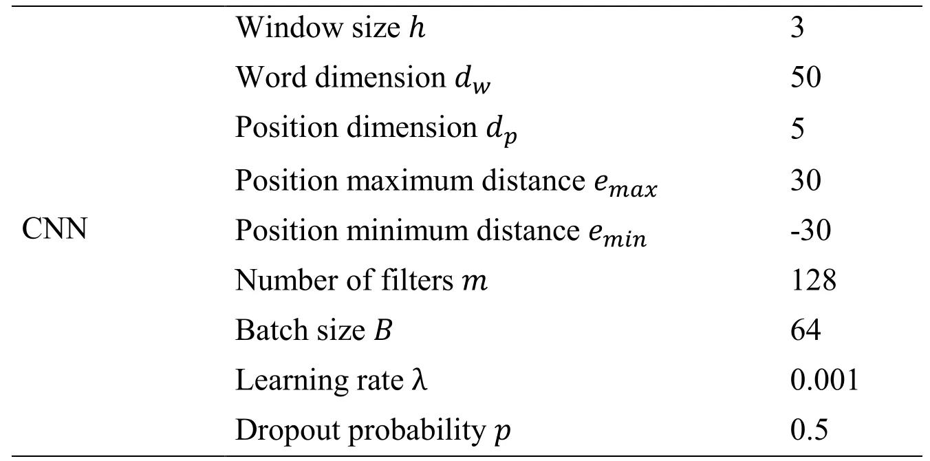
Table 2: Parameter settings for CNN-SVM

SVM Penalty parameter C 500 Kernel type kernel ‘rbf’ Kernel coefficient gamma 1.3 Tolerance for stopping criterion tol 0.01
3.1.3 Experiments for evaluation
We experiment with several state-of-the-art baselines.
● CNN-B: Our implementation of the CNN baseline [Zeng, Liu, Chen et al.(2015)] which contains one convolutional layer, and one fully connected layer.
● CNN+ATT: CNN-B with attention over instance learning [Lin, Shen, Liu et al.(2016)].
● PCNN+ATT: Piecewise CNN-B with attention over instance learning [Lin, Shen, Liu et al.(2016)].
● CNN: CNN model which includes one convolutional layer and three fully connected layers [Quirk and Poon (2017)].
● CNN-x: Deeper CNN model which has x convolutional layers.For example, CNN-9 is a model constructed with 9 convolutional layers and three fully connected layers [Feng, Guo, Qin et al.(2017)].
● CNN+PCA: Our proposed SVM model combined PCA.
● CNN+SVM: Our proposed SVM model combined CNN.
We evaluate our models on the widely used NYT freebase larger dataset [Riedel, Yao and Mccallum (2010)].NYT freebase dataset includes 522K training sentences, which is the largest dataset in relation extraction, and it is the only suitable dataset to train our model.
3.2 Corpus description
This dataset containing a training set of 522,611 sentences and a testing set consisting of 172,448 sentences can be regarded as a large amount of English news text data.We can use this dataset to train and test our models.The dataset contains 52 predefined relationship types, which means that we can extract these 52 types of relationships from English news texts.
3.3 Experimental results and analysis
The feature extraction step is implemented by the PCA method and the CNN method, and the relation classification process uses the SVM as the classifiers.In this process, the parameters of the SVM are set to be optimal and remain unchanged, and the layer settings of the CNN and the n_components for PCA are changed.Observe precision (P) and recall (R) on the training and testing sets.
In this experiment for PCA, we control the n_components value of the PCA algorithm to switch between 100, 200, 300 and 400, thereby extracting feature vectors of dimensions 100, 200, 300 and 400 from the original input data.The relation extraction is performed by using these feature vectors as inputs to the SVM.The results obtained by this experiments on the training set and the test set are shown in Tab.3.

Table 3: Test results when n_components for PCA is different
According to Tab.3, we can find that the features extracted by PCA can be used as effective input for SVM.Moreover, between 100 and 400, when n_components takes a value of 300, a relatively better relation extraction efficiency is achieved.
In the experiment for CNN-SVM, the excitation function is the ReLU function, and the maximum pooling strategy is selected.The experiment refers to the work of Huang et al.[Huang and Wang (2017)].The level of CNN is shallow and all convolution filters have a height which is same with the sentence matrices’ height.And these convolution filters have different weights.Every 128 filters correspond to a convolutional layer in the CNN, which can construct a 128-dimensional vector.When different numbers of convolution layers are set, feature vectors of different dimensions are obtained.In this experiment, several tests were carried out, and finally, when the number of convolutional layers was 1 to 3, the best results under the optimal SVM parameters are shown in Tab.4.

Table 4: Test results when the number of convolution layers for CNN is different
According to Tab.4, it can be found that in the range of 1 to 3, when the number of convolution layers is gradually increased, the P value and R value also slightly increase.There is an excellent performance of a P value of about 98.3% on the training set and about 61.3% on the testing set.
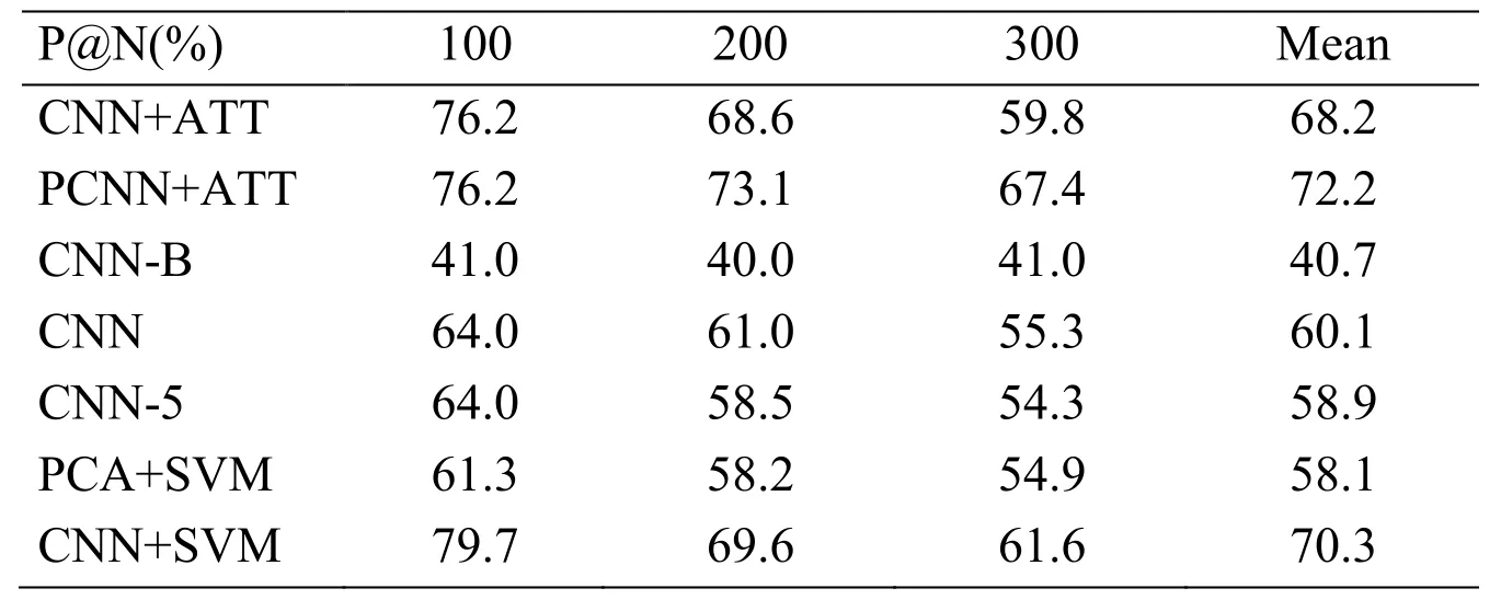
Table 5: P@N for relation extraction with different models.Top: models that select training data.Bottom: models without selective attention
In Tab.5, we compare the performances of our models to state-of-the-art baselines.We show that our CNN+SVM outperforms all models.According to the data in the table, we can find that the performance of our CNN+SVM model is similar to that of the PCNN+ATT model.For the more practical evaluation, we compare the results for precision@N where N is small (1, 5, 10, 20, 50) in Tab.6.We observe that our CNN+SVM model dominates the performance when we predict the relation in the range of higher probability.The features extracted by CNN help the SVM classifiers to better understand the meaning of the sentences and extract the relation.Besides, our PCA+SVM model also has a reasonable score, but it is not good enough to be a good choice.
In our relation extraction experience, we have two important observations:
● The SVM classifiers can make use of the feature vectors extracted by the CNN to classify the relationships and achieve good results.
● The feature vectors from CNN are better than the vectors from PCA.
● The combination of CNN and SVM can avoid the occurrence of overfitting.

Table 6: P@N for relation extraction with different models where N is small.We get the result of PCNN+ATT using their public source code
4 Conclusion
In this paper, we introduced two methods of supervised relation extraction and applied them to the field of English news, one combined SVM with PCA while the other combined SVM with CNN.We showed that CNN can extract high-quality feature vectors form the sentences for SVM.PCA was also an acceptable approach to extract the feature vectors, but it still had a large gap compared to CNN.With the support of feature vectors from CNN, the performances of SVM were significantly improved.These results suggested that SVM with CNN does have positive effects on relation extraction problems.
Acknowledgement:This work is supported by the Fundamental Research Funds for the Central Universities (HEUCFG201827, HEUCFP201839), Natural Science Foundation of Heilongjiang Province of China (JJ2018ZR1437).
References
Feng, X.; Guo, J.; Qin, B.; Liu, T.; Liu, Y.(2017): Effective deep memory networks for distant supervised relation extraction.Proceeding of the 26th International Joint Conference on Artificial Intelligence, pp.4002-4008.
Glorot, X.; Bengio, Y.(2010): Understanding the difficulty of training deep feedforward neural networks.Journal of Machine Learning Research, vol.9, pp.249-256.
Gormley, M.R., Mo, Y.; Dredze, M.(2015): Improved relation extraction with Featurerich Compositional embedding models.Proceeding of the Conference on Empirical Methods in Natural Language Processing, pp.1774-1784.
Huang, Y.Y.; Wang, W.Y.(2017): Deep residual learning for weakly-supervised relation extraction.http://www.techscience.com/books/mlpg_atluri.html.
Liu, S.; Shen, F.; Wang, Y.; Rastegar-Mojarad, M.; Elayavilli, R.et al.(2017): Attention-based neural net-works for chemical protein relation extraction.Proceeding of the 4th BioCreative.
Lin, Y.; Shen, S.; Liu, Z.; Luan, H.; Sun, M.(2016): Neural relation extraction with selective attention over instances.Proceeding of the 54th Annual Meeting of the Association for Computational Linguistics, pp.2124-2133.
Mooney, R.J.; Bunescu, R.C.(2005): Subsequence kernels for relation extraction.Proceedings of the International Conference on Neural Information Processing Systems.
Quirk, C.; Poon, H.(2017): Distant supervision for relation extraction beyond the sentence boundary.Proceeding of the 15th Conference of the European Chapter of the Association for Computational Linguistics, vol.1, pp.1171-1182.
Qu, M.; Ren, X.; Zhang, Y.; Han, J.(2017): Weakly-supervised relation extraction by pattern-enhanced embedding learning.Proceeding of the World Wide Web Conference, pp.1257-1266.
Riedel, S.; Yao, L.; Mccallum, A.(2010) Modeling relations and their mentions without labeled text.Lecture Notes in Computer Science, vol.6323, no.3, pp.148-163,
Zeng, D.; Liu, K.; Lai, S.; Zhou, G.; Zhao, J.(2014): Relation classification via convolutional deep neural network.Proceedings of COLING 2014: Technical Papers, pp.2335-2344.
Zheng, S.; Hao, Y.; Lu, D.; Bao, H.; Xu, J et al.(2017): Joint entity and relation extraction based on a hybrid neural network.Neurocomputing, vol.257, pp.59-66.
Zeng, D.; Liu, K.; Chen, Y.; Zhao, J.(2015): Distant supervision for relation extraction via Piecewise Convolutional Neural Networks.Proceeding of the Conference on Empirical Methods in Natural Language Processing, pp.1753-1762.
 Computers Materials&Continua2019年7期
- Computers Materials&Continua的其它文章
- A DPN (Delegated Proof of Node) Mechanism for Secure Data Transmission in IoT Services
- A Hybrid Model for Anomalies Detection in AMI System Combining K-means Clustering and Deep Neural Network
- Topological Characterization of Book Graph and Stacked Book Graph
- Efficient Analysis of Vertical Projection Histogram to Segment Arabic Handwritten Characters
- An Auto-Calibration Approach to Robust and Secure Usage of Accelerometers for Human Motion Analysis in FES Therapies
- Balanced Deep Supervised Hashing