Gradient Estimates for a Nonlinear Heat Equation Under Finsler-geometric Flow

ZENG Fanqi

School of Mathematics and Statistics,Xinyang Normal University,Xinyang 464000,China.

Abstract.This paper considers a compact Finsler manifold(Mn,F(t),m)evolving under a Finsler-geometric flow and establishes global gradient estimates for positive solutions of the following nonlinear heat equation

Key Words:Gradient estimate;nonlinear heat equation;Harnack inequality;Akbarzadeh’s Ricci tensor;Finsler-geometric flow.

1 Introduction

The paper studies nonlinear heat equation

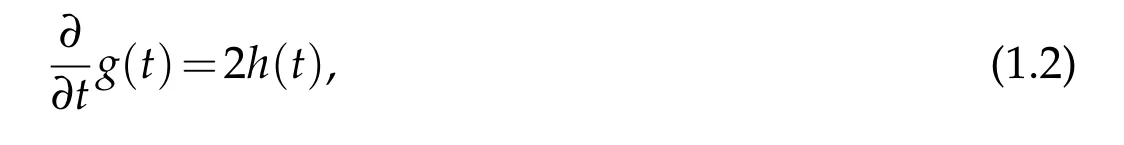
on a compact Finsler manifold(Mn,F(t),m)evolving by the Finsler-geometric flow where(x,t)∈M×[0,T],g(t)is the symmetric metric tensor associated withF,andh(t)is a symmetric(0,2)-tensor field on(Mn,F(t),m).An important example would be the case whereh(t)=-Ricij(t)andg(t)is a solution of the Finsler-Ricci flow introduced by Bao[1].Unlike the usual Laplacian,the Finsler-Laplacian Δmis a nonlinear operator.For the existence,uniqueness and Sobolev regularity of a positive global solution of the nonlinear heat equation(1.1)(in the sense of distributions),we can see[2].We will give some gradient estimates and Harnack inequalities for positive global solutions of equation(1.1).

The study of gradient estimates for the heat equation originated with the work of P.Li and S.-T.Yau[3]. They proved a space-time gradient estimate for positive solutions of the heat equation on a complete manifold.By integrating the gradient estimate along a space-time path,a Harnack inequality was derived.Therefore,Li-Yau inequality is often called differential Harnack inequality.Li-Yau type gradient estimates have been obtained for other nonlinear equations on manifolds,see for example[4-13]and the references therein.Over the past two decades,many authors used similar techniques to prove gradient estimates and Harnack inequalities for geometric flows.For instance,in[14],weakening Guenther’s curvature constrains in[15]on the boundedness of the gradient of scalar curvature in addition to the boundedness of the Ricci curvature,Liu established first order gradient estimates for positive solutions of the heat equations on complete noncompact or closed Riemannian manifolds under Ricci flows.As applications,he derived Harnack type inequalities and second order gradient estimates for positive solutions.Generalizing Liu’s work to general geometric flow,Sun[16]established first order and second order gradient estimates for positive solutions of the heat equations under general Riemannian-geometric flows.The list of relevant references includes but is not limited to[17-21].

Comparatively,there are less works on Finsler manifolds about gradient estimates of the nonlinear heat equation(1.1).To the best of our knowledge,in[22],Ohta and Sturm derived a Li-Yau gradient estimate as well as parabolic Harnack inequalities on compact Finsler manifolds. In[23],Lakzian derived differential Harnack estimates for positive global solutions to(1.1)under Finsler-Ricci flow.Later,the author and He[24]generalized and corrected Lakzian’s results under some curvature constraints.Compared to the Riemannian case,it is harder to get the gradient estimate due to some obstructions.First,the solutions of(1.1)are lack of higher order regularity.Second,Δmuhas no definition at the maximum point ofu,and thus we cannot use Finsler-Laplacian to adopt maximum principle.Last but not least,in view of nonlinear property of gradient operator,it is difficult to do the calculations.In this paper,we follow the work of Sun[16],and establish some gradient estimates for positive global solutions of(1.1)under Finsler-geometric flow(1.2),which are richer than[16,22-24].

The rest of this paper is organized as follows.

In Section 2,we first briefly review some facts and results about Finsler geometry.In Section 3,we establish space-time gradient estimates for positive global solution of(1.1),see Theorem 3.1. We also give the corresponding Harnack inequalities,see Corollary 3.1.Finally,in Section 4,we give two applications to the Finsler-Ricci flow and Finsler-Yamabe flow.

2 Preliminaries

In this section we briefly recall the fundamentals of Finsler geometry by Bao,Chern and Shen[25],as well as some results on the analysis of Finsler geometry by Ohta-Sturm[2,22].

2.1 Finsler metric

We assume thatMis ann-dimensional smooth connected manifold.LetTMbe the tangent bundle overMwith local coordinates(x,y),wherex=(x1,···,xn)andy=(y1,···,yn).AFinsler metriconMis a functionF:TM-→[0,∞)satisfying the following properties:

(i)Fis smooth onTM{0};

(ii)F(x,λy)=λF(x,y)for allλ＞0;

(iii)For any nonzero tangent vectory∈TM,the approximated symmetric metric tensor,gy,defined by

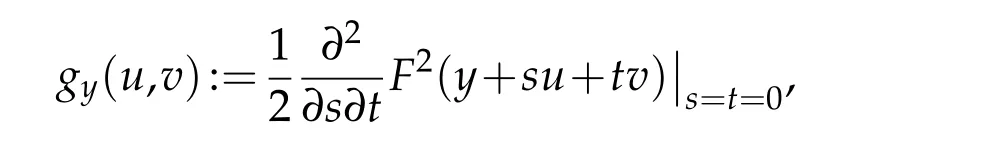
is positive definite.

Such a pair(Mn,F)is called a Finsler manifold.A Finsler structure is said to bereversibleif,in addition,Fis even.OtherwiseFis nonreversible.We say a Finsler manifold(Mn,F)is forward(resp.backward)complete if every geodesic defined on[0,a](resp.[-a,0])can be extended to[0,+∞)(resp.(-∞,0]).Compact Finsler manifolds are both forward and backward complete.By aFinsler measure spacewe mean a triple(Mn,F,m)constituted with a smooth,connectedn-dimensional manifoldM,a Finsler structureFonMand a measuremonM.

2.2 Geodesic spray and Chern connection

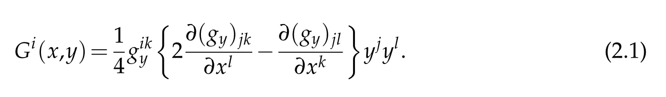
It is straightforward to observe that thegeodesic sprayin the Finsler setting is of the form,where,

For every nonvanishing vector fieldV,gij(V)induces a Riemannian structuregVofTxMvia

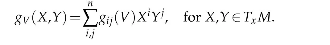
In particular,gV(V,V)=F2(V).

The projectionπ:TM-→Mgives rise to the pull-back bundleπ*TMoverTM{0}.As is well known,onπ*TMthere exists uniquely theChern connection D.The Chern connection is determined by the following structure equations,which characterize“torsion freeness”:

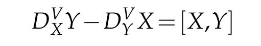
and“almostg-compatibility”

forV ∈TM{0},X,Y,Z∈TM.Here

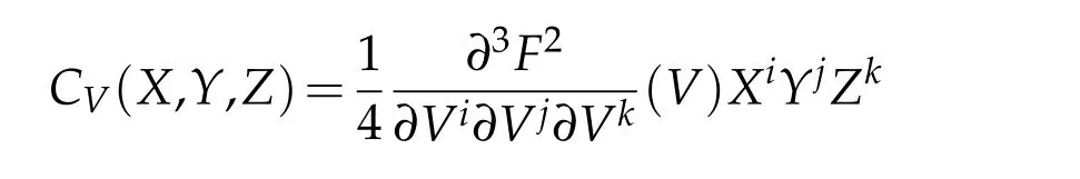
denotes the Cartan tensor andthe covariant derivative with respect to reference vectorV ∈TM{0}.We mention here thatCV(V,X,Y)=0 due to the homogeneity ofF.The Chern connection coefficients are given by

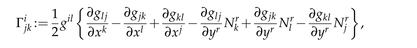
whereandgis in factgy.

2.3 Covariant derivation of tensor field

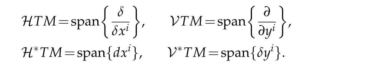
Given the coordinates{xi,yi}onTM,one can observe that the pairforms a horizontal and vertical frame forTTM,wheredenote the local frame dual towhereThen we obtain a decomposition forT(TM{0})andT*(TM{0}),

where

Letbe an arbitrary smooth local section ofThey can therefore be expanded in terms of the natural basisThe covariant derivative ofTijdenotes

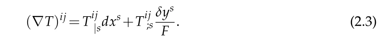
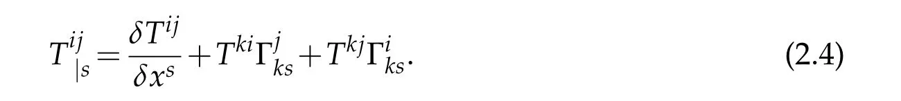
The horizontal covariant derivativedenotes

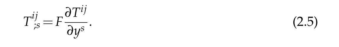
The vertical covariant derivativedenotes

2.4 Distance function

Forx1,x2∈M,thedistance functionfromx1tox2is defined by

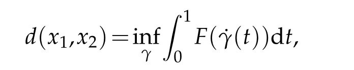
where the infimum is taken over allC1-curvesγ:[0,1]→Msuch thatγ(0)=x1andγ(1)=x2.Note that the distance function may not be symmetric unlessFis reversible.AC∞-curveγ:[0,1]→Mis called ageodesicifF()is constant and it is locally minimizing.In terms of the Chern connection,a geodesicγsatisfies

2.5 S-Curvature

Associated to any Finsler structure,there is one canonical measure,called the Busemann-Hausdorff measure,given by

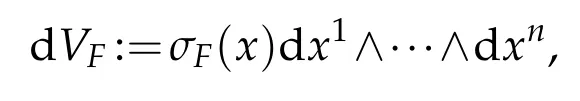
whereσF(x)is the volume ratio

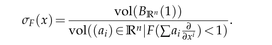
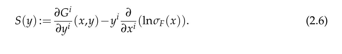
TheS-curvature is then defined as

2.6 Legendre transform,Gradient,Hessian and Finsler-Laplacian

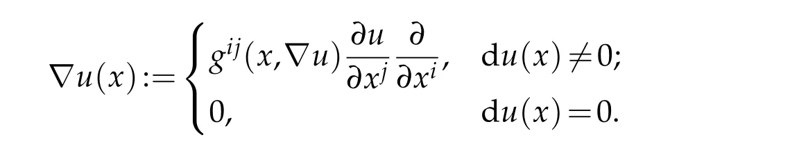
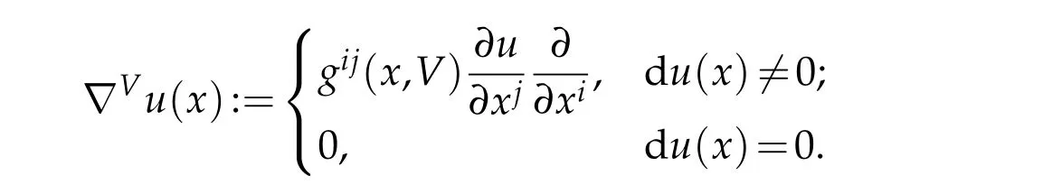
In order to define thegradientof a function,we define theLegendre transform L:TM-→T*M,asL(y)=FFyidxi,which satisfiesL(0)=0 andL(λy)=λL(y)for allλ ＞0 andy∈TM{0}.ThenL:TM{0}-→T*M{0}is a norm-preservingC∞diffeomorphism.For a smooth functionu:M-→R,thegradient vectorofuatx∈Mis defined as∇u(x):=L-1(du(x))∈TxM,which can be written as

Set.We defineforx∈Muby using the following covariant derivative

Set

Then we have

for anyX,Y∈TxM.

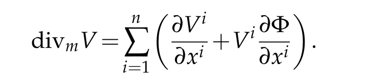
In order to define a Laplacian on Finsler manifolds,we need a measurem(or a volume formdm)onM.From now on,we consider the Finsler measure space(M,F,m)equipped with a fixed smooth measurem.LetV ∈TMbe a smooth vector field onM.In a local coordinate(xi),expressingdm=eΦdx1dx2···dxn,we can write divmVas

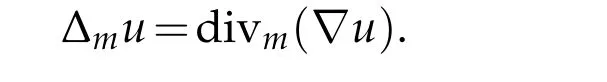
A Laplacian,which is called theFinsler-Laplacian,can now be defined by

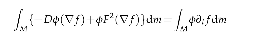
We remark that the Finsler-Laplacian is better to be viewed in a weak sense that foru ∈W1,2(M),

whereDφis the differential 1-form ofφ.

The relationship between Δmuand∇2uis that

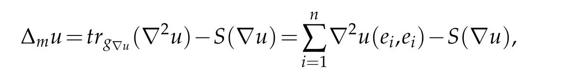
where{ei}is an orthonormal basis ofTxMwith respect tog∇u.

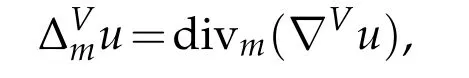
Given a vector fieldV,theweighted Laplacianis defined on the weighted Riemannian manifold(M,gV,m)by

where

Similarly,the weighted Laplacian can be viewed in a weak sense foru ∈W1,2(M).We note that

2.7 Weighted Ricci curvature

The Ricci curvature of Finsler manifolds is defined as the trace of the flag curvature.Explicitly,given two linearly independent vectorsV,W ∈TM{0},theflag curvatureis defined by

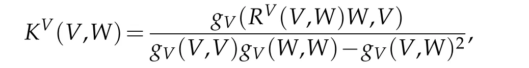
whereRVis theChern curvature(or Riemannian curvature):

Then theRicci curvatureis defined by

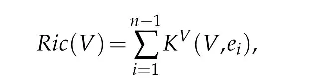
whereform an orthonormal basis ofTxMwith respect togV.

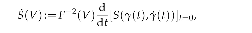
whereS(V)denotes theS-curvature at(x,V).Theweighted Ricci curvatureof(M,F,m)is defined by

We recall the definition of theweighted Ricci curvatureon Finsler manifolds,which was introduced by Ohta in[26].

Given a vectorV∈TxM,letγ:(-ε,ε)→Mbe a geodesic withDefine

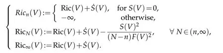
We note that the curvatureRicNis 0-homogeneous.

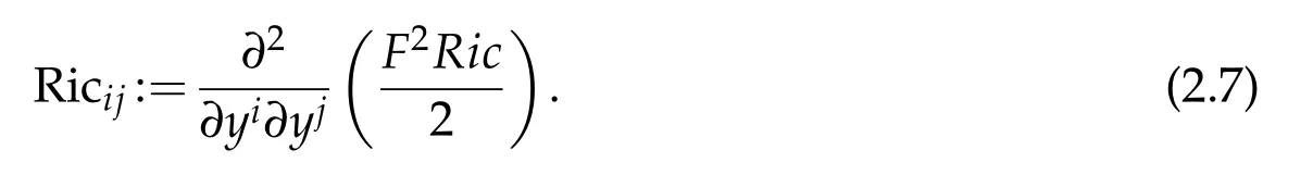
2.8 Akbarzadeh’s Ricci Tensor,Ricij

Akbarzadeh’s Ricci tensorRicijis defined as follows

We denote second order contravariant tensor of Akbarzadeh’s Ricci tensor by R,that is

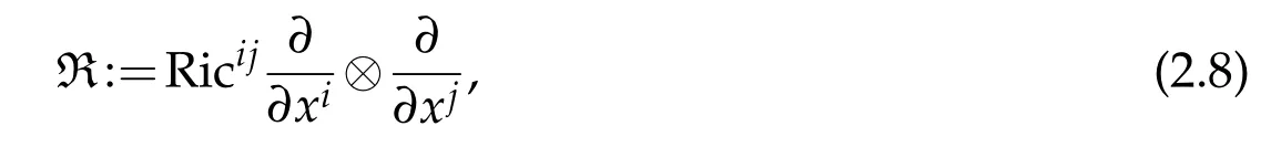
whereFor further details regarding Akbarzadeh’s Ricci tensor,see[27].

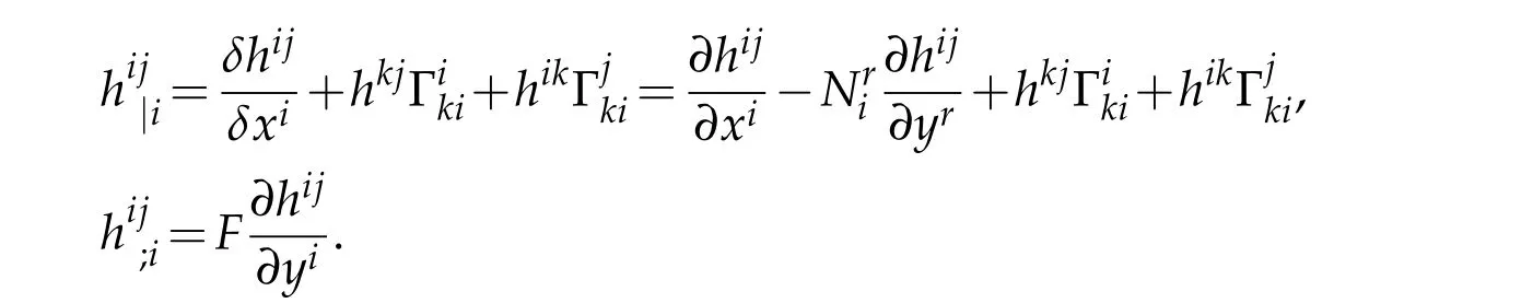
Similarly,we denote second order contravariant tensor ofhby h,that is

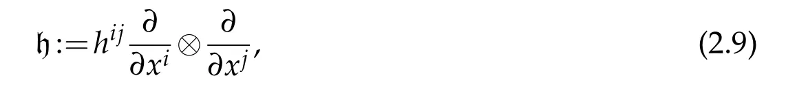
where

2.9 Bochner-Weitzenböck formula

The following Bochner-Weitzenböck type formula,established by Ohta-Sturm in[22],plays an important role in this paper.

Theorem B.([22])(Bochner-Weitzenböck formula)Δmu∈we have

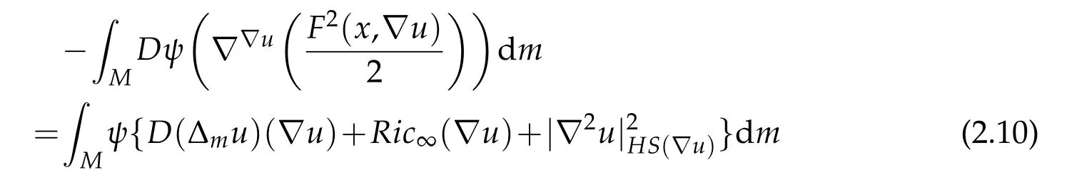
for all nonnegative functions Given u ∈C∞(M),the pointwise version of the identity is

2.10 Global solutions to ∂tu=Δmu

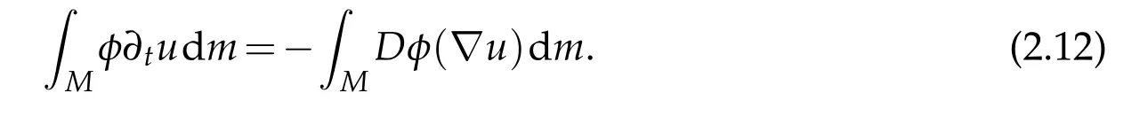
We say that a functionuon[0,T]×M,T ＞0,is a global solution to the nonlinear heat equation∂tu=Δmuif it satisfies the following:

(i)u(x,t)∈L2([0,T],H1(M))∩H1([0,T],H-1(M));

(ii)For any test functionφ∈C∞(M)and for allt∈[0,T],

3 Space-time gradient estimates for positive global solutions

Firstly,we have the following global space-time gradient estimate for the system(1.1)-(1.2).

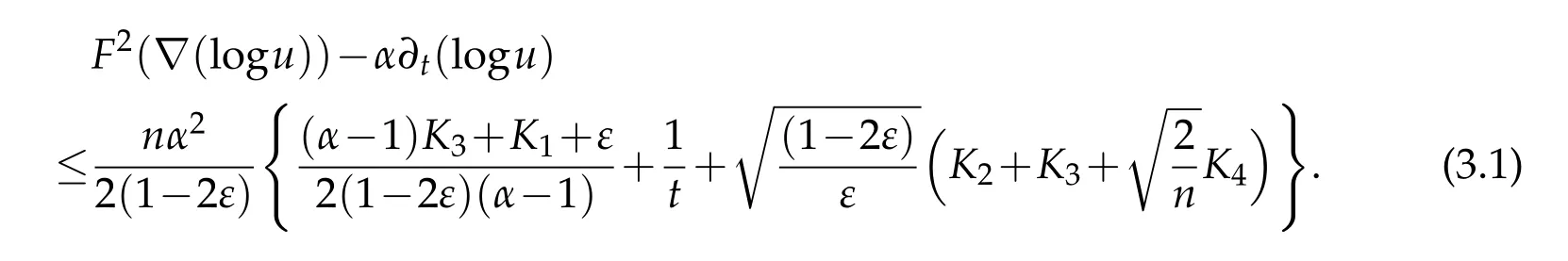
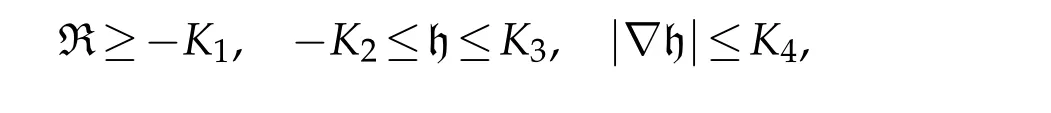
Theorem 3.1.Letbe a closed solution to the Finsler-geometric flow(1.2).Assume that there are four positive real numbers K1,K2,K3and K4such that for all t∈[0,T],

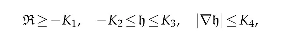
and S-curvature vanishes.Consider a positive global solution u=u(x,t)of the equation(1.1).Let f=logu.Then for any α＞1,on M×(0,T],we have

The precise definition of the Finsler measure space,R,h,|∇h|,gradient vector field∇,Finsler-Laplacian Δmand the global solution to the nonlinear heat equation(1.1)have been given in Section 2 above.

Remark 3.1.(1).Whenh(t)=-Ricij(t),(1.2)is the Finsler-Ricci flow equation.In this case our results reduce to[23,24].We also see that Theorem 3.1 covers[16,Theorem 6].

(2).The conditionS≡0 is often required in the study of Finsler-geometric flow.Since theS-curvature vanishes for Berwald metrics,our results can be applied to any Finslergeometric flow of Berwald metrics on closed manifolds(for example,see[23,28-30]).

Throughout the rest of these notes,we consider a positive solutionuof the nonlinear heat equation(1.1)on a compact Finsler manifold(Mn,F,m).The Laplacian and gradient are all with respect toV:=∇uand are valid onAlthough Chern connection coefficientis not compatible with respect tog∇f,it is torsion free. Hence,similar to Riemannian case,for a given timet,we can choose a normal coordinate system at a fixed point ofMu.We will compute at a fixed point and at this point we have

Letu(x,t)∈L2([0,T],H1(M))∩H1([0,T],H-1(M))be a positive global solution(in the sense of distributions)of the nonlinear heat equation(1.1)under Finsler-geometric flow.

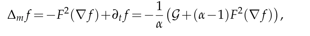
We consider the functionf:=loguwhich isH2in space andC1,αin both space and time,thenu=e f.We have

Hencefsatisfies the following equation,

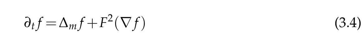
for everytin the weak sense that

for eachφ∈H1(M).From(3.3),we haveg∇f=g∇ua.e.onMuand Δm f ∈H1(M)for eacht.

To prove Theorem 3.1,we need the following several lemmas.First,we will use the following obvious lemma.

Lemma 3.1.([25])Let Ricij be a component of Akbarzadeh’s Ricci tensor and Ric be the Ricci curvature on(Mn,F,m).We have

Proceedingly,we have the following lemma.

Lemma 3.2.Let h(t)is a symmetric(0,2)-tensor field on(Mn,F(t),m).We have

derivative of hij.In particular,

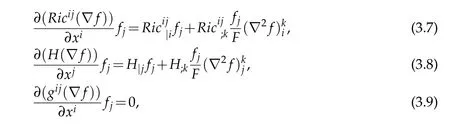
where Ricij denotes a component of Akbarzadeh’s Ricci tensor and H=gijRicij denotes the scalar curvature.

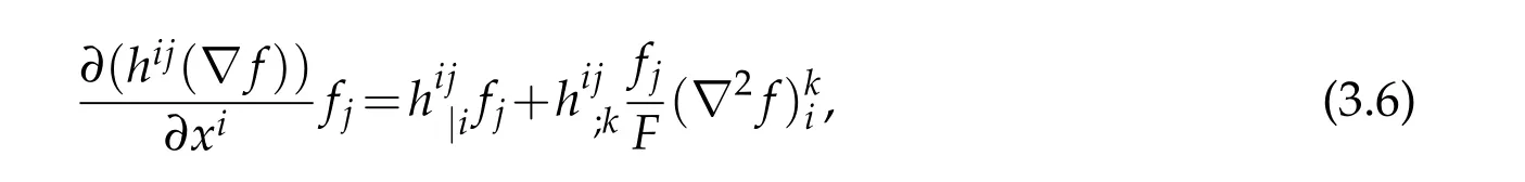
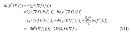
Proof.We note that

Simple differentiation gives

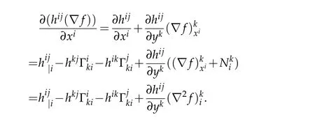
We can choose a normal coordinate system at a fixed point ofMu.We will compute at a fixed point and at this point we have

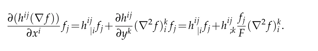
Eqs.(3.7)and(3.8)are direct consequences of(3.6).Eq.(3.9)is direct consequences of the fact

Proceedingly,we have the following lemma.

Lemma 3.3.Let(Mn,F(t),m)be a closed solution to the Finsler-geometric flow(1.2).Then we have

Proof.Simple differentiation gives

where the last equality usedandCV(V,X,Y)=0.

Let

whereα ＞1 is a constant.J(x,t)=α∂t f(x,t)lies inH1(M)andG(x,t)lies inH1(M)for eachtand is Hölder continuous in both space and time.

Proceeding,we have the following lemma.

Lemma 3.4.In the sense of distributions,J(x,t)satisfies the parabolic differential equality

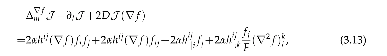
derivative of hij.

Proof.For any non-negative test functionwhose support is included in the domain of the local coordinate,we have

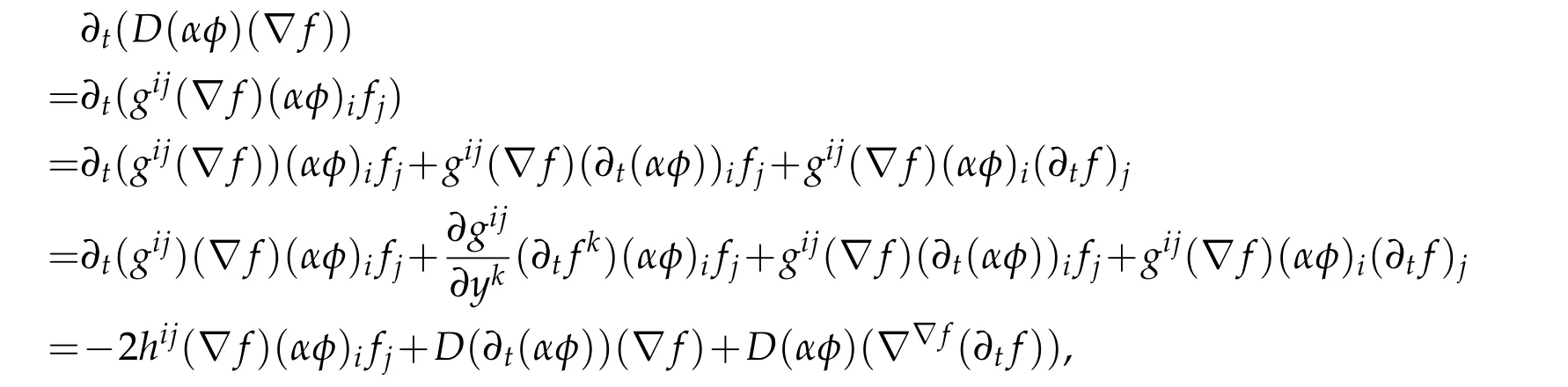
where the last equality usedandCV(V,X,Y)=0.That is,

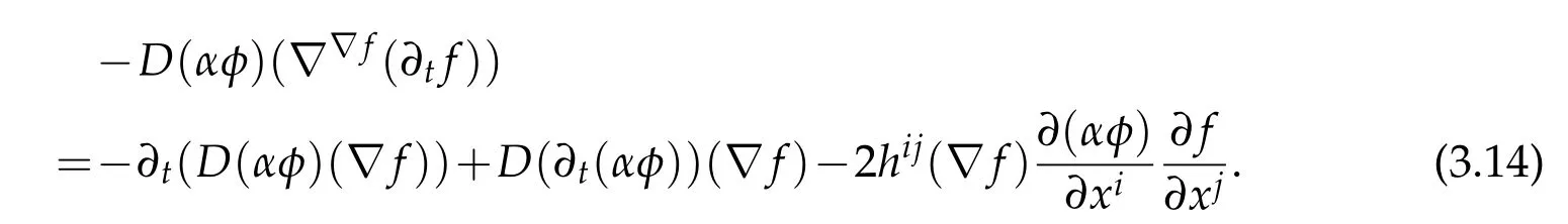
Multiplying the LHS of(3.13)byφ,integrating and then substituting(3.14),we get

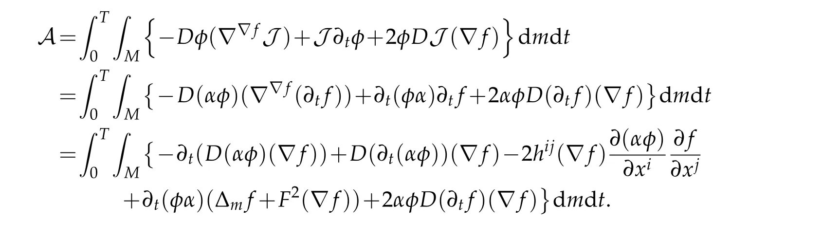
Using Lemma 3.3 and the fact that

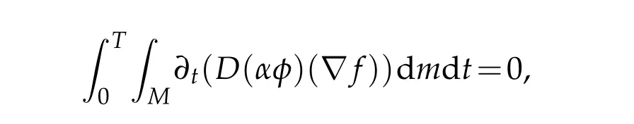
we arrive at

From(3.6)we have

This completes the proof of the lemma.

Now we can compute a parabolic partial differential equality forG(x,t)which will be the key to the proof of our Theorem 3.1.

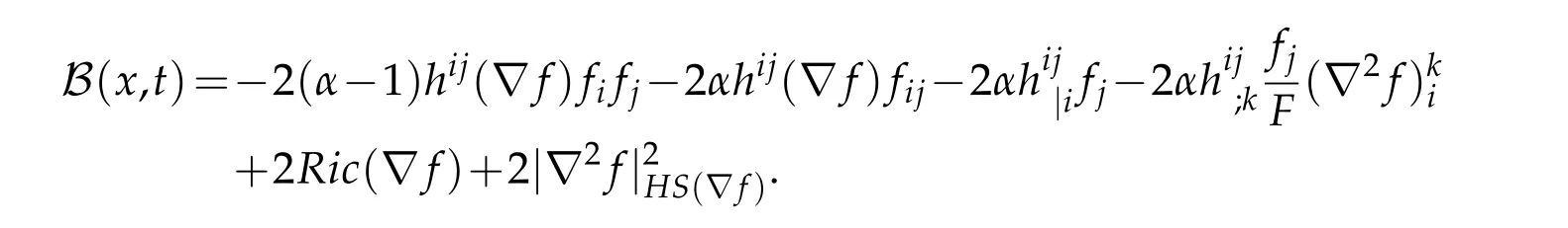
Lemma 3.5.In the sense of distributions,G(x,t)satisfies the parabolic differential equality

where

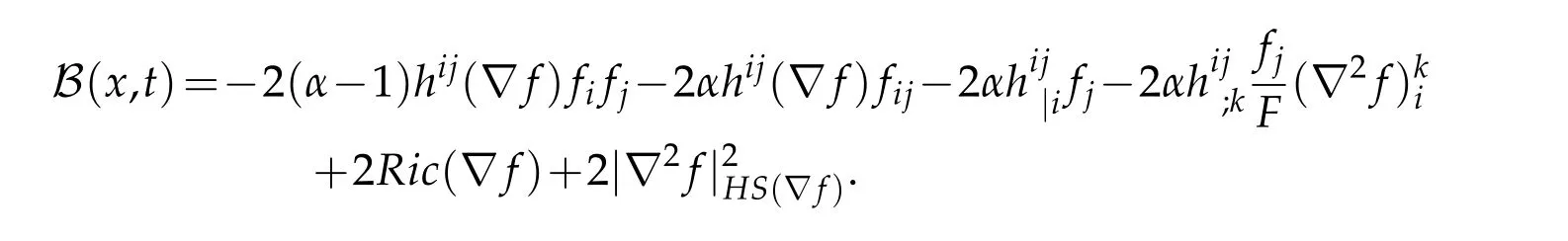
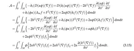
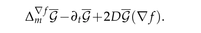
Proof.For any non-negative test functionwe compute

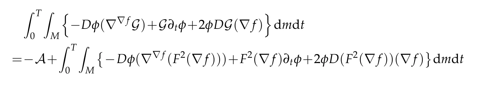
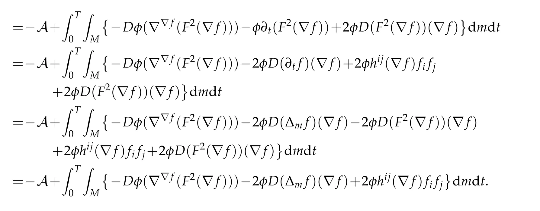
By applying the Bochner-Weitzenböck formula(2.10)and noticing thatS=0 impliesRic∞(V)=Ric(V),we have

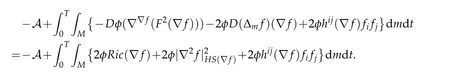
Now,substitutingAfrom(3.16),we have

Now we have all the ingredients that we need to complete the proof of Theorem 3.1.

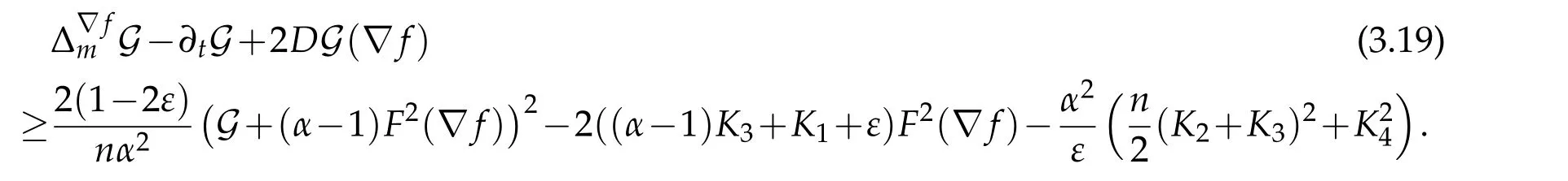
Proof of Theorem 3.1.By our assumption and(3.17),we have

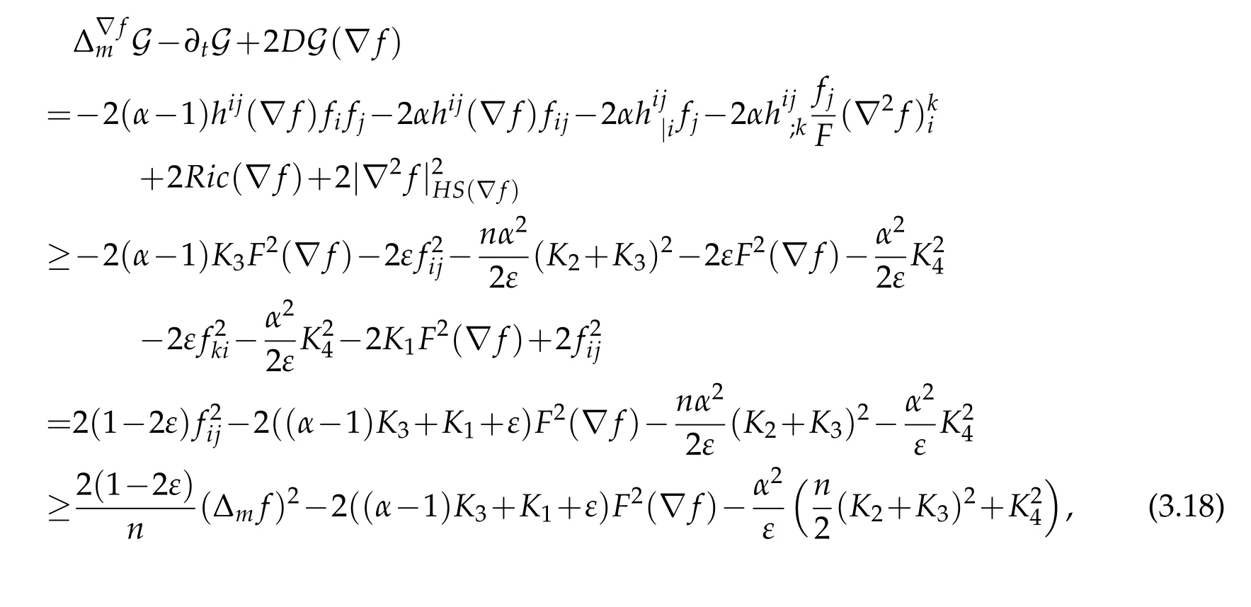
where we used

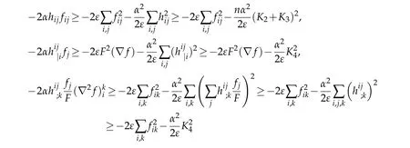
and the Cauchy inequality

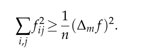
Noticing that

hence(3.18)shows

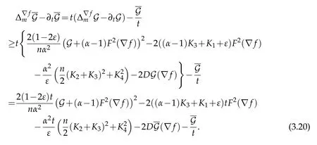
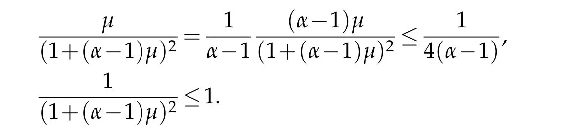
LetThen we haveμ≥0(otherwise the assertion of the theorem is trivial)and

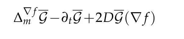
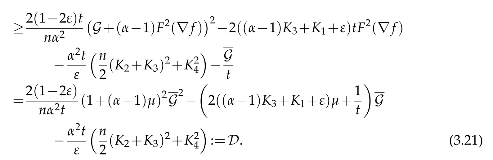
Fix arbitraryt∈(0,T]and assume thatachieves its maximum at the point(x0,t0)∈M×[0,t]and(otherwise the proof is trivial),which impliest0＞0.We shall showD(x0,t0)≤0.Assume the contrary,D(x0,t0)＞0.It would implyD ＞0 on a neighborhood of(x0,t0).Hence,according to(3.21)on such a neighborhood,the functionwould be a strict sub-solution to the linear parabolic operator

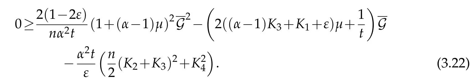
All the following computations are at the point(x0,t0).Noticing that

Solving the quadratic inequality ofin(3.22)yields

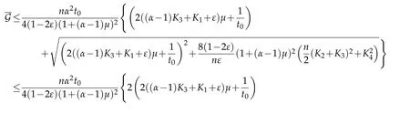
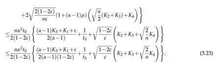
Sincet≥t0,we have

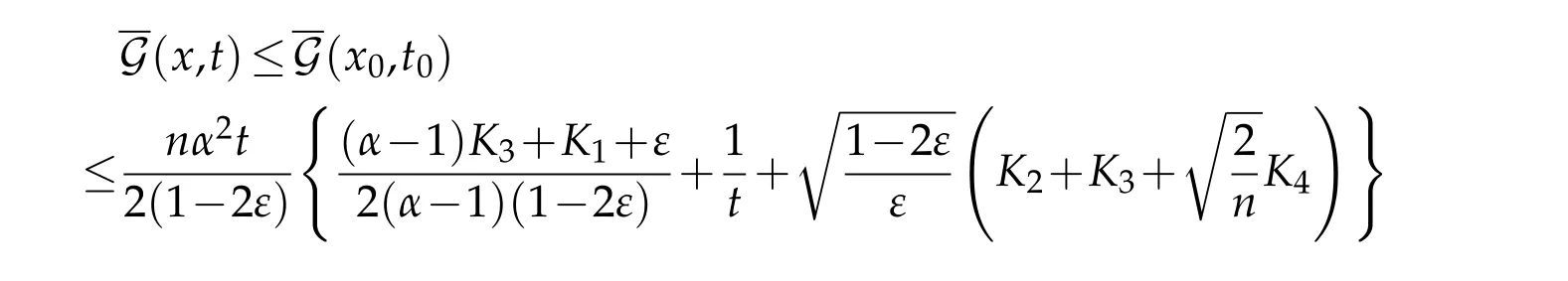
and for allx∈M,it holds that

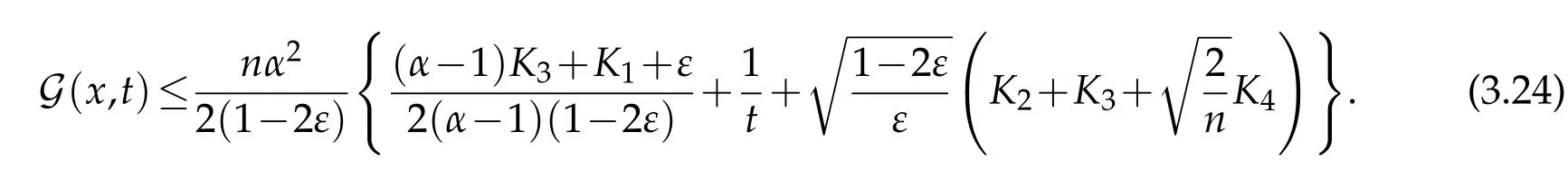
Sincetis arbitrary int∈[0,T],we obtain(3.1).Hence,we complete the proof.

Similar to[16,Corollary 8],integrating the gradient estimate in space-time as in[3],we can derive the following parabolic Harnack type inequality.

Corollary 3.1.Let(Mn,F(t))t∈[0,T]be a closed solution to the Finsler-geometric flow(1.2).Assume that there are four positive real numbers K1,K2,K3and K4such that for all t∈[0,T],

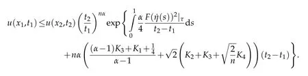
and S-curvature vanishes.Consider a positive global solution u=u(x,t)of the equation(1.1).Let f=logu.Then for(x1,t1)∈Mn×(0,T)and(x2,t2)∈Mn×(0,T)such that t1＜t2,we have

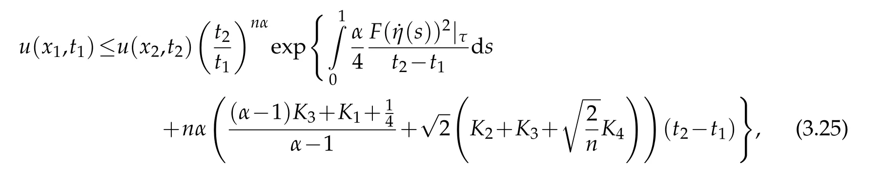
whenever α ＞1.Here η(s)be a smooth curve connecting x and y with η(1)=x and η(0)=y,and F((s))|τ is the length of the vector(s)at time τ(s)=(1-s)t2+st1.

Proof.Letη(s)be a smooth curve connectingxandywithη(1)=xandη(0)=y,andis the length of the vector(s)at timeτ(s)=(1-s)t2+st1.Choosingin(3.1)gives

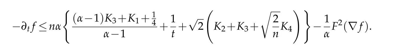
Letl(s)=logu(η(s),τ(s))=f(η(s),τ(s)).Then

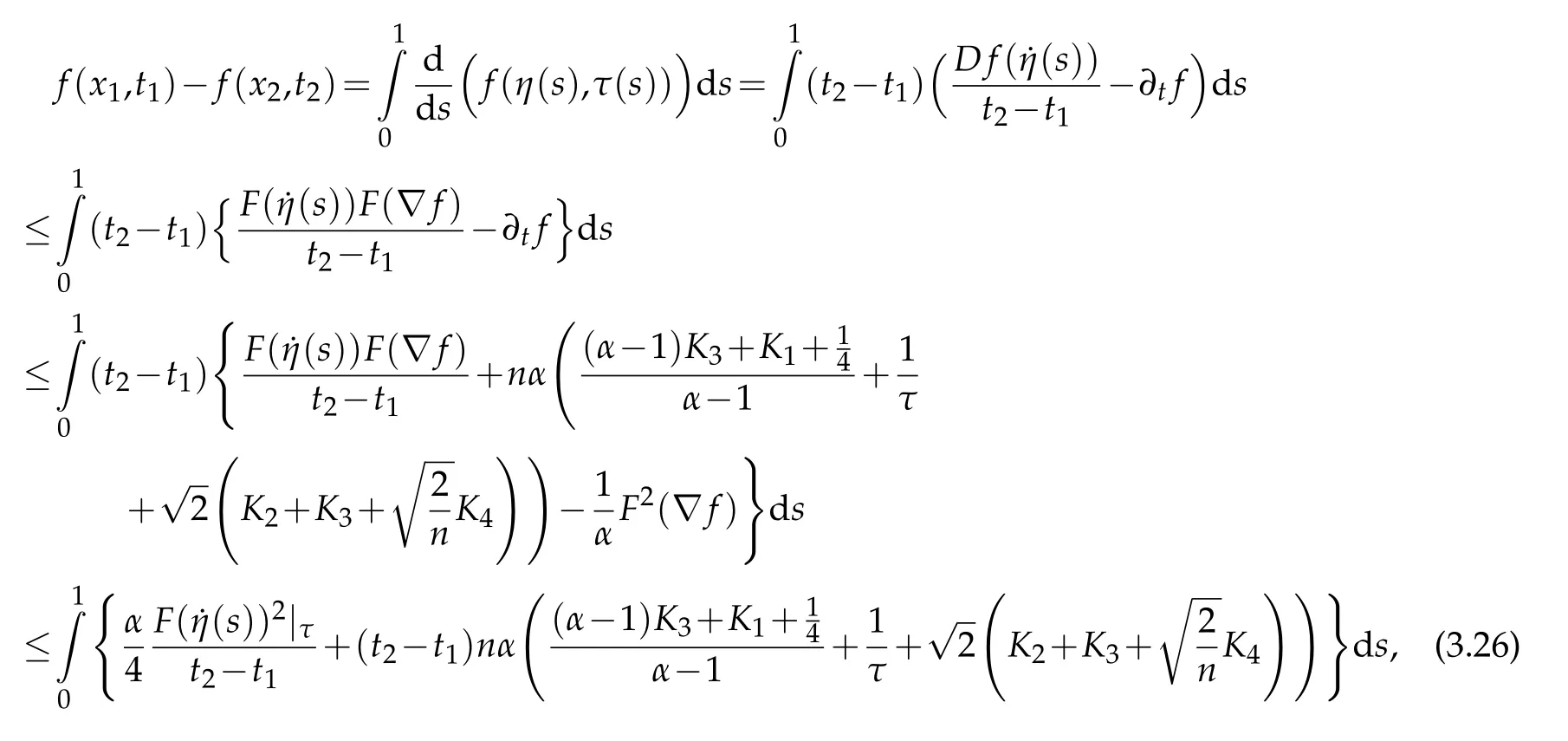
where the last inequality usedUsing(3.26),we derive

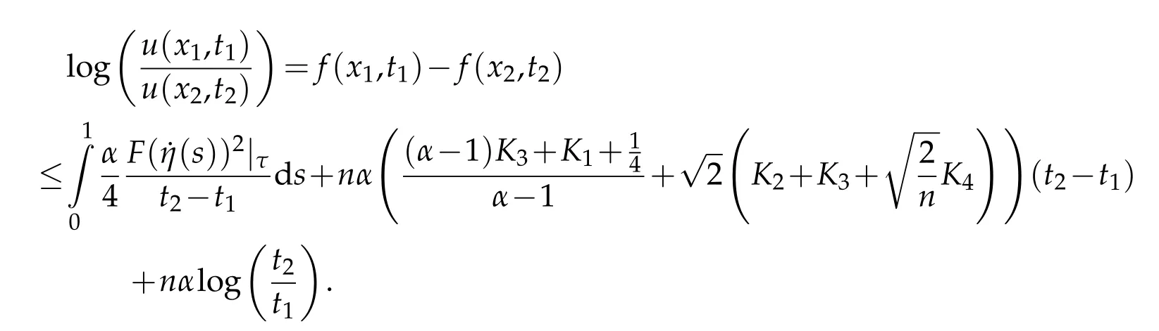
Therefore,we arrive at

4 Applications to Finsler-Ricci flow and Finsler-Yamabe flow

In this section,we apply our results to the special cases of the Finsler-Ricci flow and Finsler-Yamabe flow.

4.1 The Finsler-Ricci flow

Whenh(t)=-Ricij(t),(1.2)is the Finsler-Ricci flow equation(see[1,28,31]).In this situation our results reduced to those in[23,24].Comparing with the Riemannian case,in this case our results in Section 3 need the assumption|∇R|≤K4.Since the solutions of the nonlinear heat equation(1.1)are lack of higher order regularity,we have to compute∂t(Δm f)in a weak sense,which producesand.In order to obtain the gradient estimate,we require|∇R|bounded above.

It is worth to notice that the inequality(2)in[23]was not completely correct.In fact,due to the proof of Lemma 4.1 in[23],Lakzian thought that

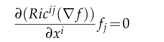
by Euler’s theorem.This means that the parabolic differential equality(43)in[23]is lack ofHowever,we compute

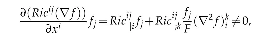
hence our results generalize and correct the work of Lakzian in[23].

4.2 The Finsler-Yamabe flow

When(1.2)is the Finsler-Yamabe flow equation

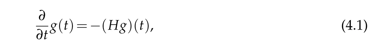
whereH=gijRicijis called the scalar curvature.For further details regarding the Finsler-Yamabe flow,see[29,32].

However,to prove our Theorem 4.1,it is enough to consider for allt∈[0,T],

andS-curvature vanishes to derive the following space-time gradient estimate for the system(1.1)-(4.1).

Theorem 4.1.Let(Mn,F(t))t∈[0,T]be a closed solution to the Finsler-Yamabe flow(4.1).Assume that there are four positive real numbers K1,K2,K3and K4such that for all t∈[0,T],

and S-curvature vanishes.Consider a positive global solution u=u(x,t)of the equation(1.1).Let f=logu.Then for any α＞1,on M×(0,T],we have

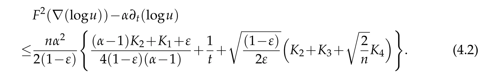
Here ε∈(0,1)is an arbitrary constant.

The proof of Theorem 4.1 is similar to the one at Section 3.We only to sketch a very simple outline of the proof.First of all,we have the following several lemmas.

Lemma 4.1.Let(Mn,F(t),m)be a closed solution to the Finsler-Yamabe flow(4.1).Then we have

Lemma 4.2.In the sense of distributions,J(x,t)satisfies the parabolic differential equality

where H|i denotes the horizontal covariant derivative of H and H;k denotes the vertical covariant derivative of H.

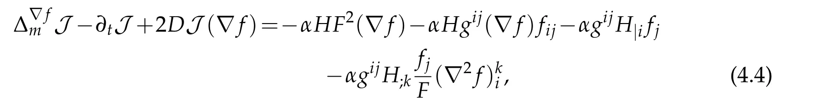
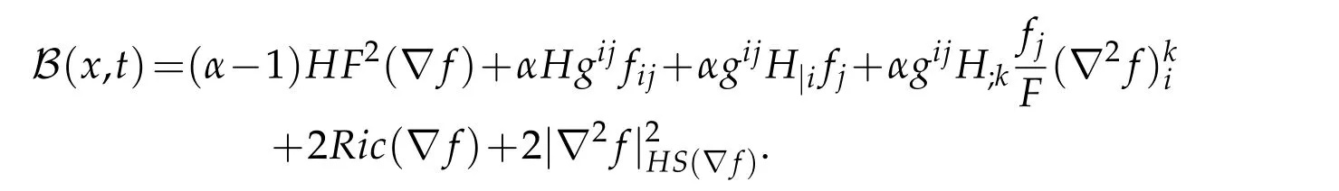
Lemma 4.3.In the sense of distributions,G(x,t)satisfies the parabolic differential equality

where

Lemma 4.4.In the sense of distributions,G(x,t)satisfies the parabolic differential inequality

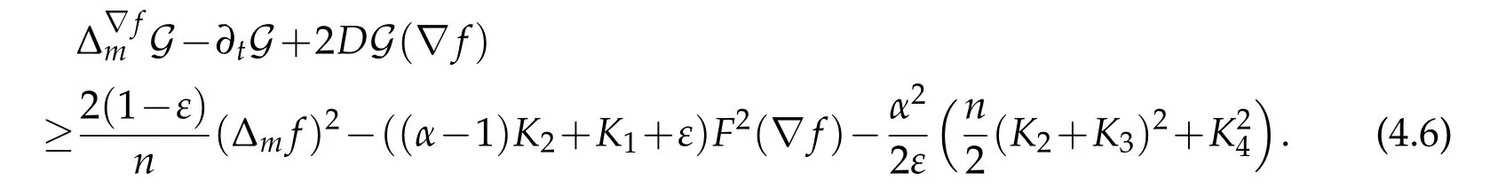
Then,using Lemma 4.4,the quadratic formula and the maximum principle,we can complete the proof of Theorem 4.1.

Acknowledgement

This work was supported by NSFC 11971415 and Nanhu Scholars Program for Young Scholars of XYNU.