
Sensor radiation interception risk control in target tracking
2020-06-28 03:03CePangGanlinShanWeiningMaGongguoXu
Defence Technology 2020年3期
Ce Pang, Gan-lin Shan, Wei-ning Ma, Gong-guo Xu
Army Engineering University, Shijiazhuang Campus, Shijiazhuang, Hebei, 050003, China
Keywords:Radio frequency stealth Target tracking Interception probability Interception risk Hungary algorithm
ABSTRACT This paper is mainly on the problem of radiation interception risk control in sensor network for target tracking. Firstly, the sensor radiation interception risk is defined as the product of the interception probability and the cost caused by the interception. Secondly, the radiation interception probability model and cost model are established,based on which the calculation method of interception risk can be obtained.Thirdly,a sensor scheduling model of radiation risk control is established,taking the minimum interception risk as the objective function. Then the Hungarian algorithm is proposed to obtain sensor scheduling scheme. Finally, simulation experiments are mad to prove the effectiveness of the methods proposed in this paper, which shows that compared with the sensor radiation interception probability control method,the interception risk control method can keep the sensor scheduling scheme in low risk as well as protect sensors of importance in the sensor network.
1. Introduction
With the application of anti-radiation weapons (anti-radiation missile, anti-radiation aircraft, radar warning receiver) [1,2] in the battlefield, active sensors (radars) are facing the threat of being intercepted and destroyed while emitting electromagnetic waves to detect targets. In order to improve the survival performance of sensors while undertaking the detection task, radio frequency stealth technology [3,4] was raised. In radio frequency stealth technology, the key point is to handle the contradiction between satisfying operational demands and reducing interception threat by controlling working parameters such as radiation power, emission time and emission time interval of sensors [5,6]. Therefore, it belongs to the scope of sensor management [7].
There are mainly two kinds of methods to achieve the aim of radio frequency stealth through sensor management.
The first method is to achieve radio frequency stealth by controlling the working parameters of sensors.At this point,reference[8,9]established the model of radiation interception probability in target tracking, and proposed the methods of controlling the minimum radiation power and the minimum emission time for controlling a single sensor.Reference[10,11]studied the problem of radio frequency stealth by designing suitable waveforms and controlling the radiation power to achieve the lowest radiation interception probability. Reference [12] achieved radio frequency steal by designing suitable radar signals, then it proposed a method of designing radar signals based on the NLFM-Costas composite signal, and the simulation proved that the signal had good results on radio frequency stealth performance.Aiming at the hardware of antenna,reference[13]designed a radar antenna with good stealth performance based on the ultra-wideband frequency selection surface.
The second method is to reduce the threat of sensor radiation interception through effective sensor scheduling methods in the process of multi-sensor cooperative detection of targets.Compared with the first method, this method was proposed later and the related theory is not as detailed as the former.At this point,under the background of multi-sensors searching and multi-targets,reference [14] established multi-objective functions with the minimum interception probability, the maximum radiation time interval and the maximum target discovery probability, and proposed a radar radio frequency stealth algorithm under joint interception threat. Reference [15] proposed a radar radiation hybrid controlling method with the minimum difference between the target tracking accuracy demand and the actual tracking accuracy as the objective function, and the simulation results performed well. In Ref. [16], the sensor scheduling methods for targeting detection and target tracking were proposed under the constraint of radiation interception probability in the background of sensor collaborative detection.Reference[17]studied the problem of radio frequency stealth in phased array radar under the background of multi-target tracking,which could effectively reduce the radiation power while ensuring the tracking quality. In Ref. [18], radiation interception was studied in the case of interference to electromagnetic interception receiver,and a new interception probability model was established. On this basis, sensors were scheduled to effectively control the interception threat. Literature [19,20]established a radiation interception threat model based on Hidden Markov theory in the case of not-knowing working parameters of the enemy’s receivers, and controlled the radiation threat in the case of target tracking, with good simulation results.
After studying the literature above, it can be seen that there exist the main following problems:
(1) Although there is much study of radiation control method on a single sensor, there is lack of research on the radiation controlling method in cluster sensor networks. Compared with a single sensor, the sensor network technology and multi-sensor collaborative detection technology can obtain higher accuracy, better performance and some other significant advantages, but there seldom has methods of controlling radiation in sensor networks. Therefore, sensor networks are facing the radiation interception threat and the threat must be reduced;
(2) The radiation control has not yet been combined with the actual operational requirements. The previous researches only control the radiation interception probability in the view of technical indicators,and they hold on the point that once the demand of target detecting precision is meet, the lower the probability of being intercepted, the better the performance is. But once it achieves the lowest limit of the interception probability, there will be no meaning of controlling it any more.At this point,it can protect the sensors of more importance at the sacrifice of the sensors of less importance from the tactical view, which means it will be a good choice that the less important sensors undertake the most radiation interception risk to protect the more important sensors in the tactical view.
To solve the mentioned problems above, this paper proposes a sensor scheduling method in combination of the sensor radiation interception risk. The rest of this paper is organized as follows. In Section 2, the concept of sensor interception radiation risk is proposed firstly,and the radiation interception probability controlling method is compared with the sensor radiation interception risk controlling method. Section 3 proposes the sensor radiation interception probability model, the cost model, and the radiation interception risk model, based on which the sensor scheduling objective function is built, with the target tracking accuracy as constraint conditions. In section 4, the Hungarian algorithm is introduced and designed to obtain sensor scheduling scheme.Before Section 6 concludes this paper, Section 5 makes some simulation experiments, which can claim the effectiveness of the method and algorithm proposed in this paper.
2. The analysis on sensor radiation interception risk
In the past papers, the “radiation interception risk control” is regarded as “radiation interception probability control”. And up to now, the definition of risk has not been clearly given. This article firstly defines the“radiation interception risk”and differentiates it with “radiation interception probability".
The risk of an event is defined as the product of the harmful event with the cost once the event occurs. Based on this concept,the definition of the sensor radiation interception risk (noted as“interception risk”) can be further obtained as the product of the sensor radiation interception probability (noted as “interception probability”) and the cost (noted as “cost”) after the sensor radiation is intercepted.
The combat situation is taken into consideration as follow:Some reconnaissance planes (targets) equipped with radiation receivers and weapons from the enemy are moving towards our defensed center.The purpose of the enemy is to detect and destroy our radars(sensors). When the targets are flying, we also want to detect and destroy them,and our sensors emit radiation in the target detection and tacking process.Once the radiation from our sensors is received by the enemy’s radiation receivers,the positions of our sensors will be acquired by the targets and they will launch missiles to destroy our sensors. The combat situation described above is shown in Fig.1.
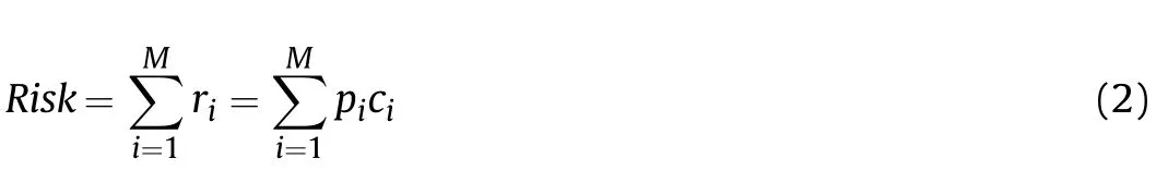
The interception risk is noted as r, and its calculation method can be provided as the definition of risk as follows.

where the variable p denotes the probability of being destroyed,and the variable c denotes the cost after the sensor is destroyed.
There are two requirements which should be satisfied to destroy a sensor for the enemy, and they are finding the positions of the sensor and hitting the sensor after they launch missiles.Thus there is the equation p = pc1pc2, where the variable pc1denotes the radiation interception probability and the variable pc2denotes the striking probability.
For the reason that this paper is mainly on the detection process and the striking process is not our focus, we assume the striking probability as“1”so as to simplify the calculation.Then there is the equation p≈pc1, and the variable p can be seen as the radiation probability.
Another advantage of regarding the striking probability as“1”is that only by doing so can be give us more space to control the risk obeying the pessimistic principle.
The“cost”can be regarded as the strategic damage caused to us after the sensor is destroyed by the strike.
For the description above,it can be seen as follows.
(1) Due to the“probability”factor,“risk”is an event that has not yet occurred but has a certain probability of occurrence.Due to “loss”, “risk” is a “harmful” event, and the smaller the value of risk is, the better it is.
(2) Compared with “probability”, “risk” takes more consideration of actual demands.If there is no“cost”,controlling the“probability” will lose its practical significance.
(3) Compared with “cost”, “risk” is an event that has not yet occurred, and once the harmful event occurs, “risk” will be converted to“cost".
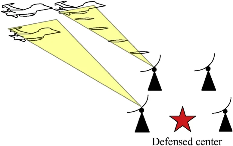
Fig.1. The combat situation.
The difference and connection between “interception risk control” and “interception probability control” are as follows.
(1) When a single sensor performs the target detection task,the risk control and probability control are equivalent to each other.
It can be seen from Eq. (1) that when a single sensor emits electromagnetic waves to obtain observations, since the cost is a constant value, the interception risk is proportional to the interception probability, and the interception risk control and interception probability control can be mutually converted.
(2) When multiple sensors are performing the same target detection tasks in cooperation, there are some essential differences between risk control and probability control.
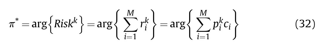
Assume that there are M sensors in the networks used to detect and track targets,and the risk value of the sensor networks can be calculated by:
where the variable Risk denotes the total interception risk of the sensor network;the variable ridenotes the interception risk valued of sensor si; the variable pidenotes the interception probability of sensor si; the variable cidenotes the cost once the sensor siis intercepted and destroyed.
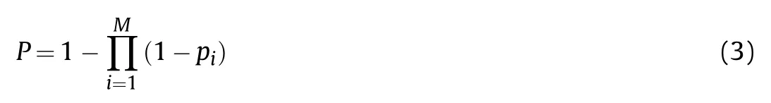
The joint interception of the sensor network can be calculated by:
When there is M = 2, assume that there are c1=0.1 and c2= 3,and the relationship of the interception risk value and the interception probability is shown in Fig. 2.
From Fig. 2, it can be seen that in the interception risk control method, different sensors are in the different strategic positions,and the more important sensors’destroying brings more cost than the less important sensors’destroying.It can reduce the risk values by applying the less important sensors to undertake more emission to reduce the risk value. However, in the interception probability control method, the emission is shared equally by each sensor in the sensor network, then the total risk value increases.
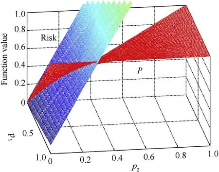
Fig. 2. Comparisons of two controlling method.
3. The radiation interception risk control model
In this section, the general sensor radiation interception probability model in the case of target detection is established firstly;Secondly,the target tracking accuracy estimation method based on UKF is introduced;What’s more,on the basis of the models above,the radiation risk control model is put forward to serve as the basic method of sensor scheduling.
3.1. The sensor radiation interception probability model
It is assumed that targets detected by our sensors carry electromagnetic radiation receivers on themselves. At time instantk,when the radiation from sensor siis intercepted by target tj, there are two requirements to be satisfied as follows:
(1) The radiation must be the same as the enemy’s receiver in frequency (pf), space (ps), and time (pt) [8];
(2) The radiation can be acquired and detected,and that is to say,the power (pd) should be big enough [9]. Then the sensor radiation interception probability can be calculated by:

Aiming at the first interception requirement, the analysis is as follows [8,9].
(1) For the radiation receiver installed in target tj, the window function is noted aswhere the variableis the time spent on scanning the whole frequency fjfor the receiver, and the variable Bjis the transmission band of the receiver.
(2) For target tj,the window function of the scanning antenna iswhere the variablesandare the rotation rate and beam width of the antenna.
(3) For sensor si,the window function of impulse signal iswhere the variablesandrepresent the pulse repetition interval and pulse width respectively.According to the window functions defined above, it can be expressed by the Poisson distribution as follows.

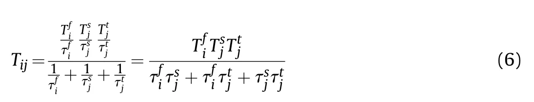
where the variable Tsis the dell time of the electromagnetic wave;there isand the variable Tijis the average coincidence period of three windows.
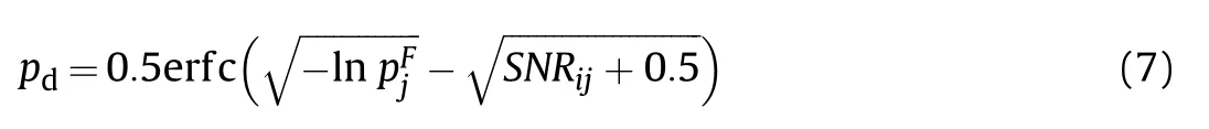
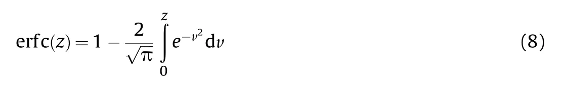
For the second interception requirement,the variable pdcan be calculated by Ref. [17]:
It is assumed that other parameters of each radiation receiver are the same except for the radiation time,radiation power and the distance between the target and the radar.In order to simplify the calculation, the signal-to-noise ratio is calculated as follows [21].
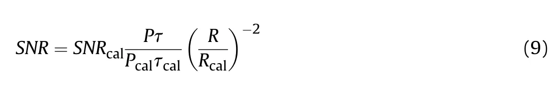
where the variable τ is the radiation time with the power P; the variable R is the distance of the sensor and the target;the variable SNRcalis the radio of signal to noise when the distance of a target and a sensor is Rcalwith the radiation power Pcaland the radiation time τcal.
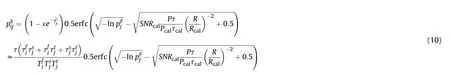
It is assumed that the electromagnetic wave time emitted by the sensor is equal to the dwell time of the electromagnetic wave shinned on the target.At time instant k,the radiation interception probability of sensor siintercepted by target tjis as follows.
At time instant k- 1, the cumulative radiation interception probability of sensor siis noted as,and at time instant k,after sensor siemits radiation to detect target tj,the cumulative radiation interception probability can be changed to
3.2. The cost model
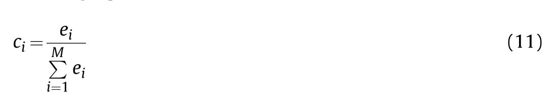
In this paper,the cost brought to us after the sensor is destroyed is determined by the importance of the sensor in the sensor network. A sensor network is shown in Fig. 3.
In Fig. 3, the damage of blue sensor node will not affect the connectivity of the whole sensor network, while the damage of green sensor node will prevent the gray nodes from communicating with the commanding center. Therefore,it can be seen that the damage of different sensors will cause different costs to our sensor network.
In this paper,the cost once a sensor is destroyed can be regarded as the strategic position of the sensor in the sensor network.
The sensor network model is noted as G(V,L),where the variable V is the set of sensor nodes,and the variable L is the set of the edges.
The adjacency matrix is noted as, where there is aij∈{0,1}, and when aij= 1, sensor siand sensor sjcan communicate with each other, or they cannot communicate once there is aij= 0. The degree of sensor siis defined as
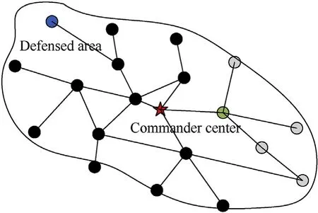
Fig. 3. The sensor network.
In this paper,sensors have the same working performances,and the importance degree of sensor sican be calculated by the following equation.
3.3. The target tracking precision based on UKF
At time instant k, the moving state of a target can be noted as Xk=[xk, ˙xk,yk, ˙yk]T.
The state transition matrix is denoted aswhere the variable T is the sampling time, and there is T =1 s in this paper.
At time instant k+1,the moving state of the target transmits as follows.

where the variable W is the process evolution noise, and each component follows a Gaussian distribution with a mean of 0; the variable Q is the noise covariance matrix, and there isin this paper, where variables σxand σyare the power spectral density of the noise.
At time instant k+1,the observation of sensors can be noted as follows.
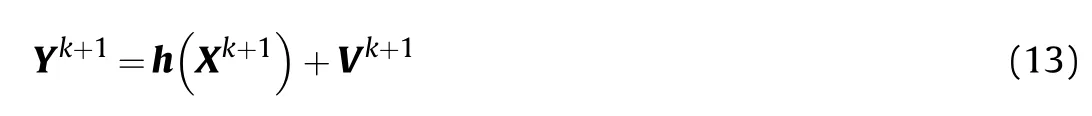
where the variable Vk+1is the observation noise, and follows a Gaussian distribution with a mean of 0; the variable
In this paper,the target tracking precision is defined as follows.

The target tracking accuracy is calculated by Unscented Kalman Filtering (UKF) [22]. UKF is based on Unscented Transformation(UT).
There is the n-dimension variableand m-dimension variable.

where the variable g( ) is the nonlinear transformation function.
The purpose of UT is to obtain the statistical property of y according to the statistical property of x, and then the statistical property of nonlinear function propagation can be obtained.There are 2n+1 sigma points χi, and the rules of selecting sigma and their coefficients are as follows.
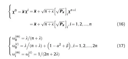
where the variable λ=α2(n+κ)-n can determine the distance of sigma points andthe variable α is usually set to a small integer(104≤α<1); the variable κ is usually set to 0 or 3- n; for a Gaussian distribution, β=2 is the optimal value; there is, where[]irepresents the ith column.
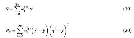
These sigma points propagate through a nonlinear function g( ),and then there is:

The mean value and variance of y are calculated by:
The calculation is based on UKF and the estimation of target tracking precision is as follows.
(1) Initialization
Step 1 Provide the initial filtering conditions:,P0,Q0,and R0.
At time instant k = 1,2,3,…, loop from Step 2 to Step 8.
(2) Prediction
Step 2 According to the variablesandat time instant k- 1, select variablesand ω0,ω1, …,ω2n.
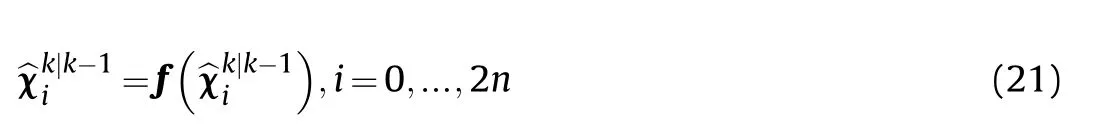
Step 3 Carry out nonlinear transformation according to the target state model, and there is:
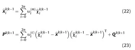
Step 4 The mean value and the covariance of the state prediction are as follows.
(3) Update
Step 6 Carry out the nonlinear transformation according to the measurement model, and it is:
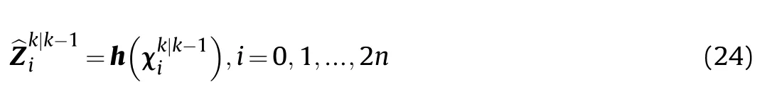
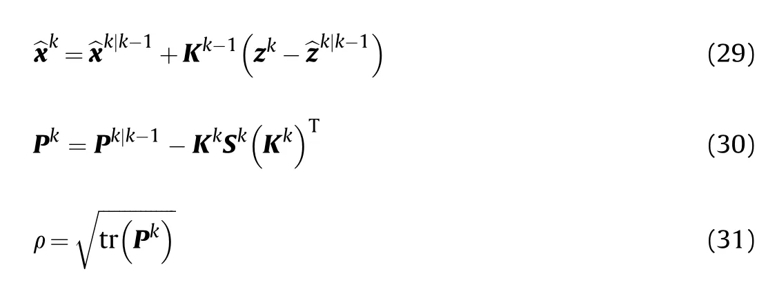
Step 7 the mean value of measurement prediction,information covariance, mutual covariance between state and measurement and filtering gain are as follows.
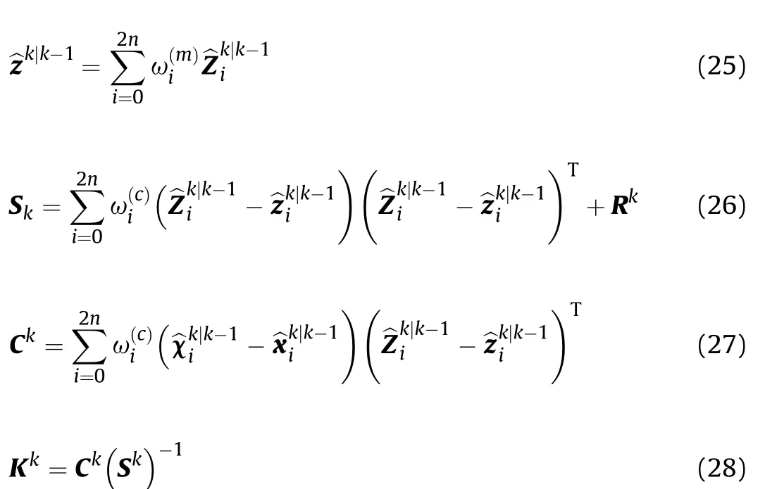
Step 8 at time instant k, the posterior state estimation mean value, covariance matrix, and target tracking precision are as follows.
3.4. The radiation risk control model
In this paper, there are M sensors in the network used to tracking N targets.At time instant k,the sensor scheduling scheme is noted aswhere=1 denotes that sensor siis used to tracking target tj, otherwise, it denotes not.
At time instant k,the optimal sensor scheduling scheme can be calculated by:
The constraints are as follows.
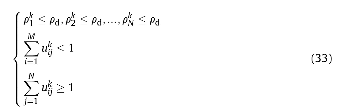
where the variable ρdis the demand of target tracking precision,and the variableis the target tracking precision of target tj.
In sensor scheduling, in order to obtain an effective solution,there are some other rules to obey as follows.
(1) If all sensors cannot meet a target’s tracking accuracy requirement, the sensor with the best tracking accuracy is selected to track the target, and the sensor is no longer selected by other targets;
(2) If two or more targets compete for one sensor in the first condition, the sensors shall be selected according to the principle of the minimum interception risk,and other targets will select their sub-optimal sensors.
4. Algorithm design
Assign M sensors to N targets, and when there is M ≥N, there arekinds of sensor scheduling schemes,which belongs to the NP (Non-deterministic Polynomial) hard problem. Optimization algorithms should be designed to obtain sensor scheduling schemes in order to adapt to the complex and varied battlefield environment.
There are some optimization algorithms such as the traversing method, the Hungarian algorithm [23], the greedy algorithm [24],the swarm intelligence algorithm(for example,the particle swarm optimization algorithm [25]), and the distribution method (for example,the game theory method[26]).Since the latter two kinds of methods are approximately optimization algorithms, the calculation results may be different from the actual optimal value, but the greedy algorithm and the traversing algorithm have obvious deficiencies in the calculation speed, this paper adopts the Hungarian algorithm which has fast calculation speed and the optimal solution result.
The Hungarian algorithm is based on the theory raised by the Hungarian mathematician D.Konig[27],and it can be used to solve the assignment problem. This paper regards the sensortarget allocation problem as the assignment problem,but the basic Hungarian algorithm needs to be transformed to some extent.The solving steps of the improved Hungarian algorithm matching the optimization background of this paper are as follows.
Step 1: Construct an adjacency matrix. For target tj, when sensor sican satisfy the target tracking precision demand,there is bij=,otherwise,there is bij=∞.If there is no sensor to satisfy the target tracking precision demand,then the optimal sensor is noted as s*and there is b*j=1 in the matrix B.For the reason that there is M ≥N in this paper, the matrix B must be expanded to a M× Mmatrix and the values are set to 0 in the column N+ 1× M.
Step 2:Each element at matrix B subtracts the smallest element at the element’s row, and the new matrix is noted as B;
Step 3:Transform elements in row of the matrix B’.Find the row where there is only one zero, and note the zero as “○”, then note the other element in its column as “ノ”. Transform elements in column of the matrix B’.Find the column where there is only one zero, and note the zero as “○”, then note the other element in its row as “ノ”.
Step 4:If there is zero noted as“○”at each column,then jump to Step 7, otherwise jump to Step 5;
Step 5: If there is any free zero in the matrix, select the row where there is the fewest number of zeros which are not noted,and operate on the zeros following the rules:
Compare the number of zeros in column where each zero is located at, and note the zeros where the number of zeros is the smallest as “○”, then note the other elements in the row and column of the zero as“ノ”.Take the actions above until all zeros are noted,then jump to Step 7, otherwise, jump to Step 6;
Step 6: If there is no free zero in the matrix and the number of zeros noted as “○” is smaller than N, note the column, where there is no zeros marked as “○”, as “☆”. Then mark the row where there are zeros noted as“ノ”as“☆”in the column which has been marked as“☆”.Underline the rows which are marked as “☆” in horizontal lines, and underline the column which are not marked as “☆” in ordinate lines. Find the smallest values among the non-covered elements by lines and note it as Δ.Each element which is noted as “☆” in column subtracts Δ , each element which is noted as“☆”in row adds Δ,then jump to Step 2;
Step 7:Mark the zero as 1,and the other elements are marked as 0, then the 0-1 and M×N matrix is Uk.
End the algorithm.
5. Simulations
In the simulation, there are 10 sensors in the sensor network and their coordinates are as follows: s1(20,20), s2(30,30),s3(100,52), s4(58,120), s5(69,36), s6(47,117), s7(150,210),s8(180,42), s9(123,85), s10(142,100).
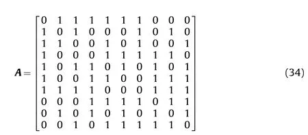
The communication relationship between sensors is as the matrix A shows.
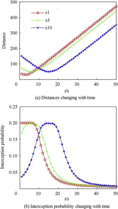
Fig. 4. The relationship of interception probability and distance.
Five targets are moving in straight lines.And their motion statesare as follows:
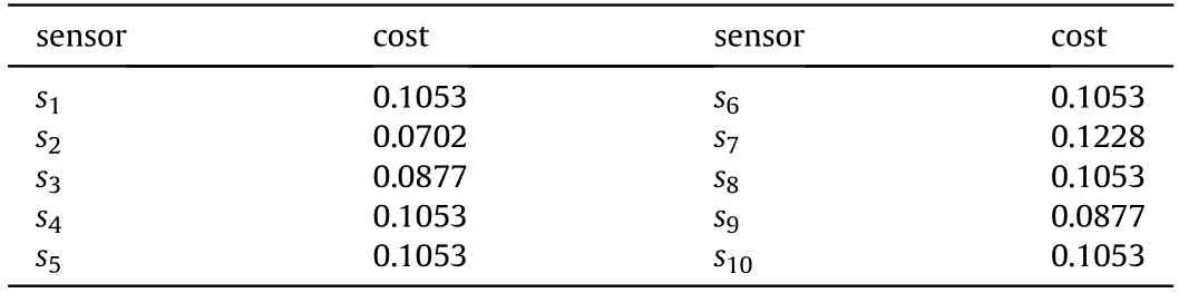
Table 1 The cost value of sensors.
5.1. Simulation on the radiation interception model
The sensor radiation interception probabilities are calculated according to Eq. (10). When target t3moves, the curves of the interception probabilities of sensors s1, s3and s10are shown in Fig. 4.
It can be seen from Fig. 4 that when target t3moves, the radiation interception probability by the target to the sensors decreases with the increase of the distance between the target and sensors.In the process of sensor scheduling, under the condition of meeting the requirement of target tracking precision,sensors which are far away from the target should be selected firstly to track the target,so as to reduce the interception probability.
5.2. Simulation on the cost model
The sensor cost values are calculated according to Eq. (11), and the calculation results are shown in Table 1.
It can be seen from the matrix A and Table 1,that the more one sensors connected by one sensor,the more important the sensor is in the sensor network,and more cost are will be brought after the sensor is destroyed.
5.3. Simulation on the calculation of sensor scheduling schemes
The improved Hungarian algorithm proposed in this paper is used to calculate the sensor scheduling scheme.The target tracking precision is set to ρd= 100. At time instant k = 0, sensors are scheduled to track targets,and the sensor scheduling schemes are calculated by the improved Hungarian algorithm (denoted as algorithm 1),the particle swarm optimization algorithm(denoted as algorithm 2), and the traversing algorithm (denoted as algorithm 3).50 Monte Carlo experiments are carried out and the calculation result is shown in Fig. 5.
In Fig.5,the traversing algorithm can get the optimal solution by comparing the performance of all alternative sensor scheduling schemes, but the convergence rate is slow. The particle swarm optimization algorithm has struck into the local optimization and cannot obtain the best scheme.Compared with the two algorithms,the improved Hungarian algorithm proposed in this paper can obtain the same scheduling scheme and risk value with traversing algorithm,and the convergence rate of the Hungarian algorithm is the fastest.
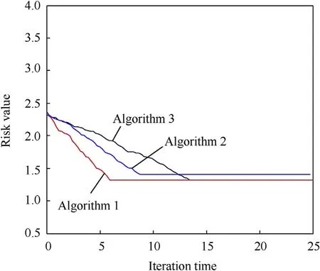
Fig. 5. The comparison of algorithms.
There are two reasons for the simulation results of Fig.5.On the one hand, the Hungarian algorithm calculates the best solution through optimization rules and the steps of analysis are finite. In contrast,the other two algorithms obtain the best scheme iteration by iteration,and if the best solution is not gotten,the iteration will not stop. So the convergence rates of them are slower than the Hungarian algorithm.On the other hand,the Hungarian algorithm can calculate the best scheme through theoretical analysis and matrix transformation. The best one must be obtained by the Hungarian algorithm,however,the other two algorithms search for the optimal scheme by comparing all solutions in each circle of iteration.If the best one is not contained in the compared solutions,it will be missed. The particle swarm optimization algorithm has struck into the local optimum as the blue curve shows in Fig. 5.
The optimal sensor scheduling scheme is as follows:t1- s2,t2-s5, t3- s8, t4- s1, t5- s10.
5.4. Simulation on sensor scheduling when targets move in straight lines
In time period k:[0,25],the sensor scheduling method based on interception risk proposed in this paper (denoted as method 1) is adopted to schedule sensors to track targets. Meanwhile, it is compared with the sensor scheduling method(denoted as method 2) based on interception probability. The improved Hungarian algorithm proposed in this paper is used to calculate the sensor scheduling schemes. The comparison of calculation results is shown in Fig. 6.
The target flight paths and sensor distribution are shown in Fig. 6(a); Curves of mean tracking precision of 5 targets changing with time are shown in Fig. 6(b); Curves of instantaneous interception risk values changing with time are shown in Fig. 6(c);Curves of cumulative value of interception risk changing with time are shown in Fig. 6(d); The curves of sensor scheduling schemes changing with time using the interception risk controlling method are shown in Fig. 6(e). The curves of sensor scheduling schemes changing with time using the interception probability controlling method are shown in Fig. 6(f).
It can be seen from Fig.6(b)that both of the two kinds of sensor scheduling methods can meet the demands of target tracking precision, but combined with Fig. 6(c), (d), (e), and (f), some other conclusions can be obtained as follows: In the Interception risk control method,the risk values keep obviously lower,and sensor s7of the most importance in the sensor network has been scheduled for only 3 times. However, in the interception probability control method,the sensor s7has been scheduled for 10 times.The results above can illustrate that while maintaining the low risk values;the interception risk control method can protect the sensors of more importance at the sacrifice of the less important sensors by making them undertaking more radiation.
5.5. Simulation on sensor scheduling when a target moves in
To make further study on the proposed sensor scheduling method and illustrate its effectiveness, the method has also been applied to the scene of multiple maneuvering targets tracking.
The simulation scene and experiment results are shown in Fig.7.
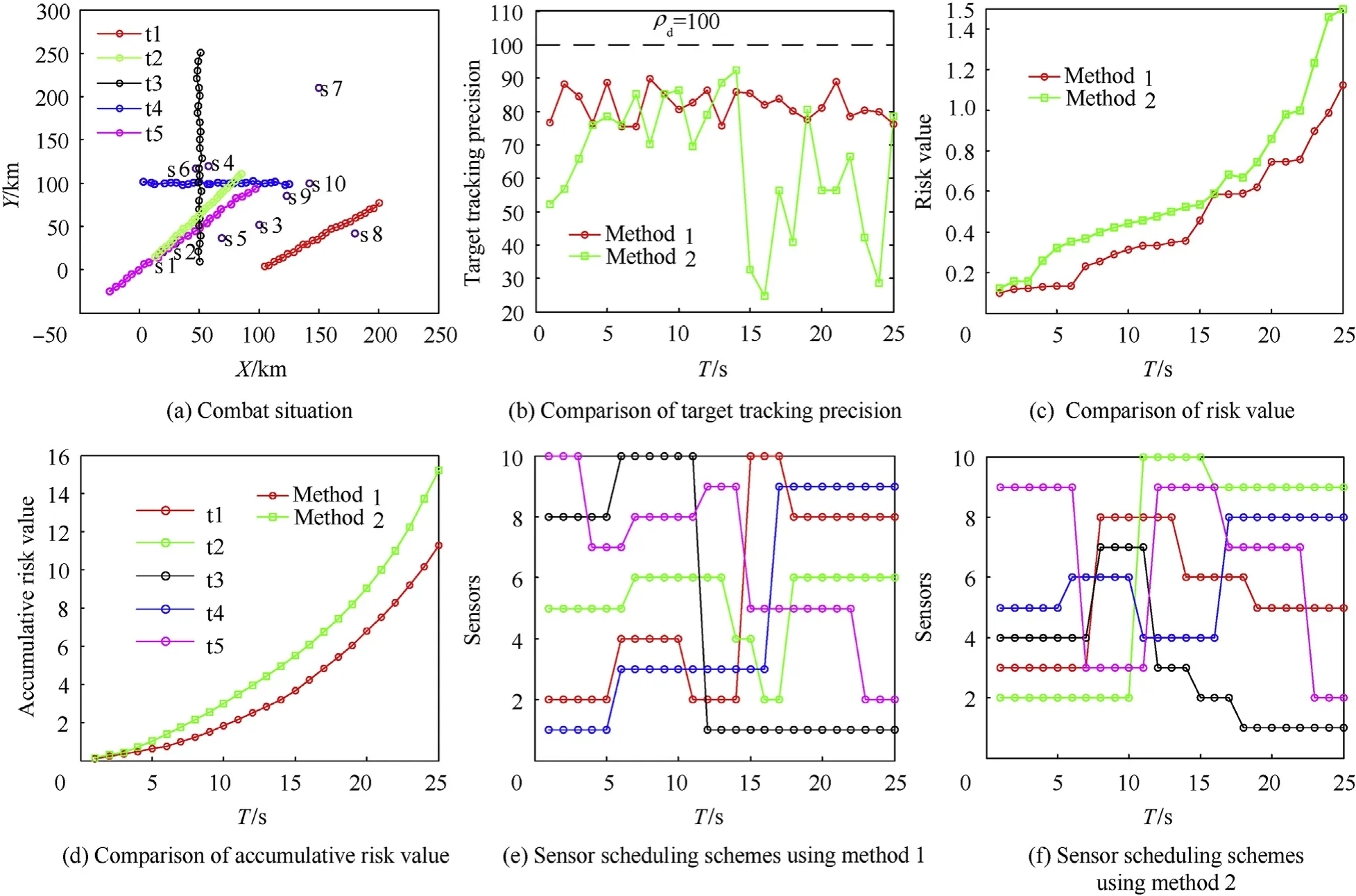
Fig. 6. Comparison of sensor scheduling methods when targets are moving in straight lines.
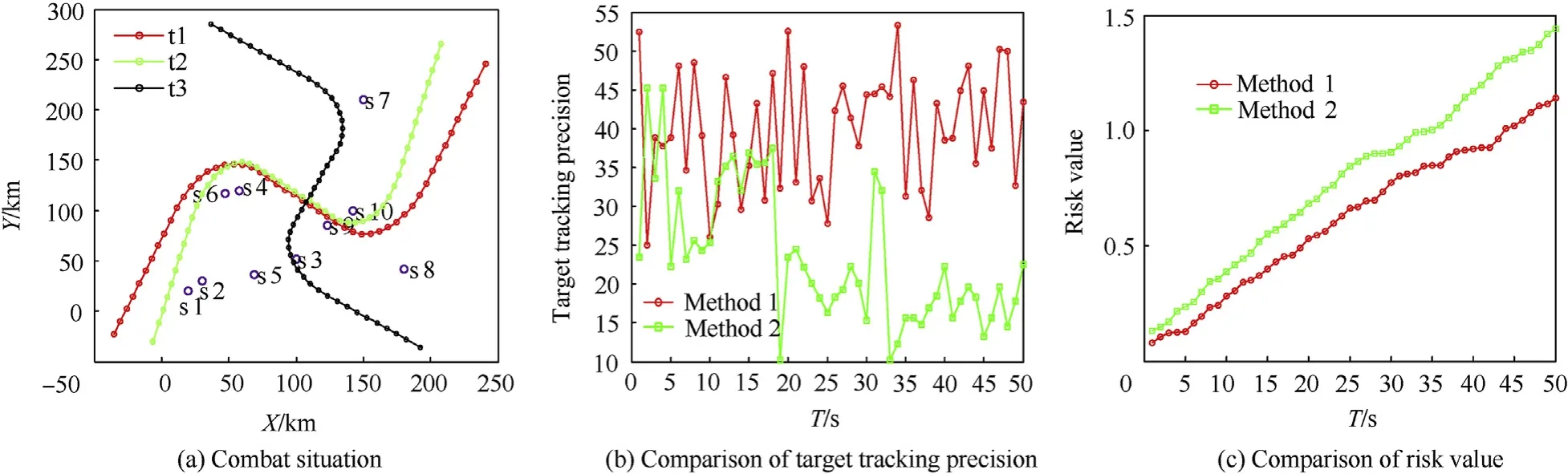
Fig. 7. Comparison of sensor scheduling methods when in multiple maneuvering targets tracking.
The target flight paths and sensor distribution are shown in Fig. 7(a); Curves of mean tracking precision of 3 targets changing with time are shown in Fig. 7(b); Curves of instantaneous interception risk values changing with time are shown in Fig. 7(c).
It can be seen that in the scene of multiple maneuvering targets tracking,the interception risk based sensor scheduling outperforms the interception probability based sensor scheduling method in interception risk with lower values in almost time instants from Fig.7(c),although the interception probabilities may not as good as the interception probability sensor scheduling method shown in Fig. 7(b). The probability is only one hand to increase the risk values,and if the cost is small,the risk values still keep pretty low,which means that it can protect the more important sensors with more cost in the network at the sacrifice of the sensors of less importance.
6. Conclusion
In this paper, the risk theory was applied to the field of radio frequency stealth and sensor management.Firstly,the definition of risk was provided, and then the sensor radiation interception risk was put forward. What’s more, the interception risk control and interception probability control were compared,and the feasibility of this method was analyzed theoretically. Secondly, to calculate the interception risk, the model of sensor radiation interception probability and the cost once the interception occurs were established. On the basis of the models above, the sensor scheduling objective function based on risk control theory was established to achieve the minimum interception risk with the constraint of target tracking accuracy.Then the Hungarian algorithm was introduced to obtain sensor schemes from the objective function. Finally simulations were made, and the results showed that the proposed interception probability model, the cost model, the sensor scheduling model based on risk control and the improved the Hungary algorithm were all effective. Especially, by using the method proposed in this paper,not only the sensor scheme with the minimum risk value could be obtained, but also the sensors of importance were effectively protected at the same time. Risk control is an important portion in combats. Besides sensor radiation interception, there are still some other kinds of risk, for example, in target detection, if there is a target but the detection result is ‘no’, the target will be missed and attack us, bringing some inevitable cost.The product of the target missing probability and the cost can be defined as the target detection risk according to the definition of the risk in this paper. Similarly, in target tracking, the risk can be called target losing risk, and in target recognition, the risk can be called target recognition risk. In the future work, all of the risk controlling methods will be studied in detail.
Declaration of competing interest
This paper has no conflict of interest with others.
Acknowledgement
This article is funded by Chinese national natural science foundation (61573374).
- Defence Technology的其它文章
- Statistical variability and fragility assessment of ballistic perforation of steel plates for 7.62 mm AP ammunition
- Texture evaluation in AZ31/AZ31 multilayer and AZ31/AA5068 laminar composite during accumulative roll bonding
- Local blast wave interaction with tire structure
- Research and development of training pistols for laser shooting simulation system
- Summed volume region selection based three-dimensional automatic target recognition for airborne LIDAR
- A novel noise reduction technique for underwater acoustic signals based on complete ensemble empirical mode decomposition with adaptive noise, minimum mean square variance criterion and least mean square adaptive filter