老龄化债券在累积和分配阶段的固定缴款养老金中的作用(英)

1 Introduction

To make wealth reallocation throughout the whole life and sustain consumption after retirement,pension fund is an important financial instrument for individuals. Typically,according to diあerent settings of contribution and benefit,there are two principal types of pension fund: defined benefit (DB) plan and defined contribution (DC) plan.For a DB pension scheme, the benefit paid after retirement is explicitly fixed by the contract in advance, while the contribution is adjusted based on the wealth to keep the fund in balance. However, for a DC pension plan, the contribution is predetermined,while the benefit depends on the contribution and the return of investment.

Generally, a pension plan consists of an accumulation (contribution) phase, which is the period before retirement, and a decumulation (distribution) phase, which is the period after retirement. There are lots of researches concentrating on optimal investment problems during both phases. For the contribution phase, for instance, Yao et al[1]investigated an optimal investment problem under the mean variance criterion.For the distribution phase, for example, Zimbidis and Pantelous[2]considered an asset allocation problem, as well as the optimal payment with the target of a certain wealth at the terminal time.

Longevity risk has recently attracted increasing attention from both academic and practical aspects. It is the risk of uncertain aggregated mortality, i.e., the risk that the aきliate lives longer than the pension sponsor’s expectation. As for the longevity risk management,the ground-up hedging strategy and the excess-risk hedging strategy were studied by Cox et al[3]. Unfortunately, not all kinds of longevity risk can be hedged for the nonparametric mortality model by the method of natural hedging, see Zhu and Bauer[4]. In addition, Wang et al[5]provided an alternative approach to investigate longevity risk for small populations. Other updated studies on longevity risk can be found in [6,7].

In order to establish a relationship between financial risks and actuarial risks,longevity bond is introduced as a kind of financial instruments,whose interest is equal or proportional to the survival rate of a given population. A detailed analysis of Swiss Re mortality bond (issued in December 2003) and EIB/BNP longevity bond (announced in November 2004) was given by Blake et al[8]. In addition, Barbarin[9]applied the Heath-Jarrow-Morton approach to price longevity bond. Later,by applying techniques developed from mortgages and credit risk areas, Wills and Sherris[10]investigated the securitization of longevity risk. Bauer et al[11]reviewed and compared diあerent methods of mortality-linked securities pricing in previous works. Redistribution of longevity risk is considered in the work of Boonen et al[12]when it is necessary to combine diあerent longevity-linked liabilities. More explanations on longevity bond and other kinds of longevity instruments can be found in [13].

Longevity bond has been widely used in the optimal portfolio area. Menoncin[14]investigated the role of such bond for a log-consumer-investor,and found that the value function in a market with the longevity bond is never lower than the value function of the market without it. Menoncin and Regis[15]studied the pre-retirement consumption and portfolio selection problems, and the result showed that investors optimally invest a large fraction of wealth in the longevity bond in the preretirement phase. Again in a market with longevity bond, Kort and Vellekoop[16]analysed the existence of the optimal consumption and investment strategies.

Longevity risk management is meaningful in a DC pension scheme. If a pension member lives longer than the expectation of the sponsor,the company must pay perpetuities for more years than what expected at the beginning,thus the plan faces longevity risk.

This paper considers a DC pension plan which continuously decides the investment weights in diあerent assets, including a longevity bond and a riskless asset, in order to:1). Maximize the terminal wealth in the period of accumulation with the consideration of a minimum guarantee; 2). Maximize the terminal wealth in the period of decumulation with the consideration of uncertainty life time, respectively. The motivation of this work is to investigate whether the expected utility of wealth is increased with the investment of the longevity bond, compared with the longevity bond replaced by an ordinary bond. In order to make it convenient for comparison, this work follows the definition of the longevity bond in previous works, see, for instance, [14] or [17], but find diあerent stochastic diあerential equation (SDE) to describe its dynamic.

The rest of this paper is structured as follows: section 2 describes the demographic pattern and the financial market with a stochastic interest rate and three tradable assets which are of interest for the pension manager. Section 3 solves an optimal problem before retirement with the consideration of a minimum guarantee to the beneficiaries,and compares the cases with and without the longevity bond in the portfolio, with both closed form solutions given by solving the related HJB equations. Section 4 solves an optimal problem after retirement with the consideration of uncertain lifetime of the given population, with a comparison similar to section 3. At last, section 5 consists of the sensitivity analysis, the comparative study and a summary.

2 Model assumptions and notations

Let (Ω,F,P) be a filtered probability space with filtration F = {Ft}t≥0which is generated by a standard Brownian motion B, i.e., Ft= σ{B(s);0 ≤s ≤t}, t ≥0.Suppose that all of stochastic processes and random variables in this paper are defined on this space.

2.1 The demographic pattern

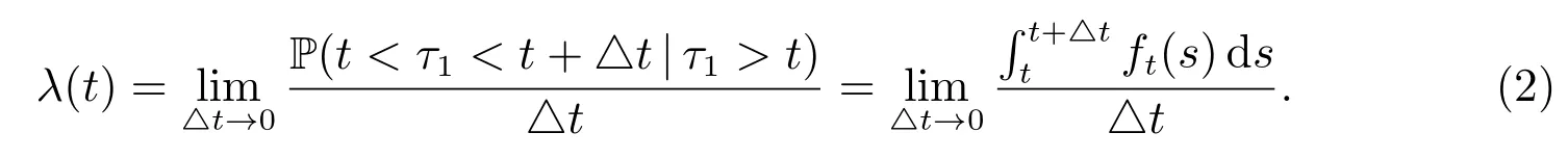
Assume that there is a given population with n individuals, whose death times are denoted by n identically independently distributed (i.i.d.) non-negative random variables τ1,τ2,··· ,τn. The conditional probability density function at time s conditional on τ1＞t(s ≥t) and the mortality rate are defined as follows

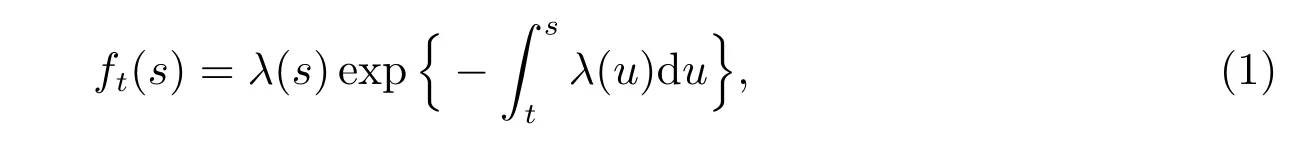
and

2.2 The financial market

The Ornstein-Uhlenbeck process introduced by Vasicek[18]is used to describe the spot rate R(t) at time t:

with an initial value R(0)=R0. All parameters are positive constants in (3).

Assume that there are three tradeable financial instruments which are of interest for the pension trustee. The riskless asset S0(t) is described by the following SDE:

with an initial value S0(0)=1.

The second asset is a zero coupon bond B(t,T0) which pays one dollar to the investor at its expiration time T0, and it is defined by

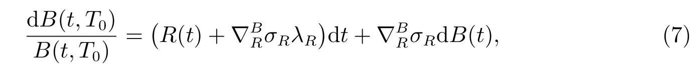
with a terminal value B(T0,T0)=1. Q is the so-called equivalent martingale measure,under which the discounted process e−R(u)duB(t,T0) is a local martingale. Applying the martingale property of the discounted process of B(t,T0), see, for instance,Menoncin[14], its evolution satisfies the following SDE

where BQ(t)is a standard Brownian motion under measure Q. By Girsanov’s theorem,dBQ(t) = λRdt+dB(t) is a Wiener process under Q, where λRis the market price of the interest rate. Thus we can obtain the dynamic of B(t,T0) under the probability measure P as

where

is the semi-elasticity of the bond price with respect to the interest rate. Since the bond reacts negatively to the interest rate,is negative. In addition, λRis also negative since the bond has a positive premium compared with the riskless asset, which makes the bond attractive to investors.

The third financial instrument is a longevity bond with the same expiration time T0, whose price at time t is denoted by L(t,T0), from which the investor gets lT0/ltunits of money at the terminal time, and there is no coupon up to time T0. With a given population whose ages are all x at the initial time 0, ltdenotes the number of people who survived to time t. By the fundamental theorem of asset pricing, we have the following relationship between L(t,T0) and B(t,T0):

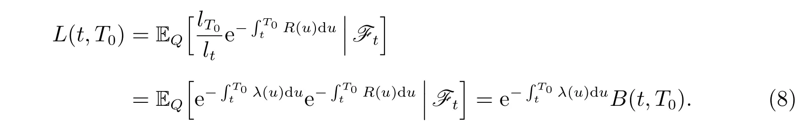
By the chain rule, the dynamics of L(t,T0) is described by the following SDE

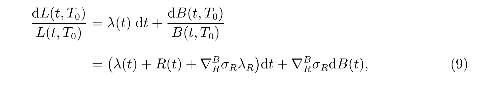
with a terminal value L(T0,T0)=1.

3 Optimal control during the accumulation phase

During the accumulation phase of a pension plan, we consider the case of a single contribution paid by the pensioner at the aきliation time 0 and there is no further contribution, while benefits are delivered into annuities at the retirement time T (T ≤T0). The corresponding optimization problem is to find the optimal investment strategy during this phase.

3.1 Fund management with investment of the longevity bond

3.1.1 Annual guarantee

As the sharing of investment risks between the aきliate and the sponsor is quite diあerent in a DC type plan (the pension member bears the majority of investment risks), there are diあerent kinds of guarantee to prevent shortfalls on benefits to make the plan more attractive to aきliates. Following the work of Devolder et al[19], Han and Hung[20]and Guan and Liang[21], we require that there is a downside protection on the pension annuity, which is denoted by

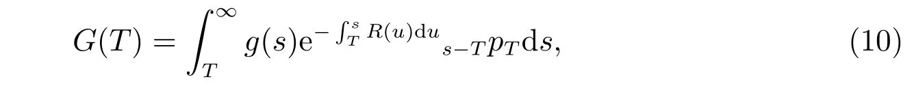
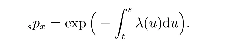
where g(t) is a deterministic function of time t which reflects inflation. Under the assumption that the present time is t,sptdenotes the probability that a life will survive at least s −t years. Mathematically,

3.1.2 Wealth process and optimization problem

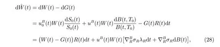
During the accumulation phase, the pension manager invests an initial contribution C0into the financial market. subsection 3.1 considers the market composed of a longevity bond and a riskless asset,in which case the market is complete. The dynamics of returns on the wealth process would be

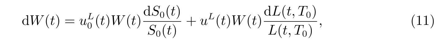
with an initial value W(0)=C0.(t) and uL(t) are weights invested into the money market account and the longevity bond, respectively. We assume that borrowing and short-selling are permitted in the context.

Definition 1A strategy uL(t) is called admissible if it satisfies the following conditions, and we denote the set of all admissible controls by Π.

1) uL(t) is progressively measurable with respect to {Ft}t∈[0,T0];

3) (11) has a unique strong solution for the initial value (0,R0,C0) ∈[0,T]×(0,∞)2.

To maximize the expected utility of the terminal fund W(T) over the guarantee G(T), we introduce the following optimization problem

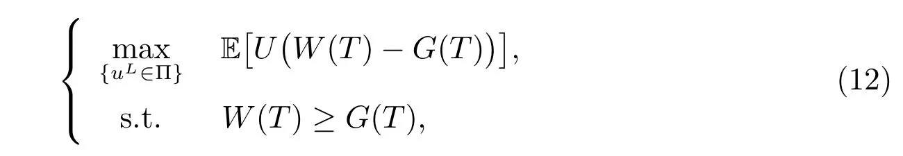
where U(x) is the utility function which reflects the sponsor’s preference. Here we consider the CRRA utility function

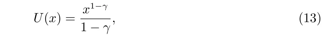
where γ is the relative risk aversion with conditions γ ＞0 and γ ̸=1.

3.1.3 Construction of an auxiliary problem

Since the optimal investment problem (12) is not a single problem, an auxiliary process is constructed in the following to transform the initial problem into a single one. The present value of the minimum guarantee is defined by

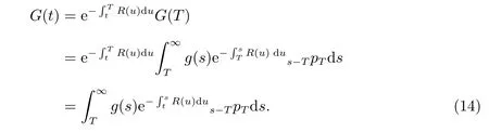
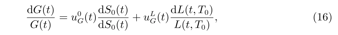
By diあerentiating, we have the dynamic of returns on G(t):

Remark 1G(t) can be regarded as a kind of financial instrument in the market,which can be totally replicated by the bank account S0(t). It is more clear in the following representation

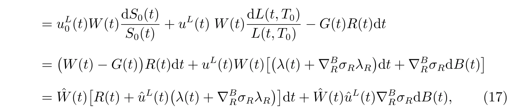
Thus the initial maximization problem(12)can be converted into a single problem as the following

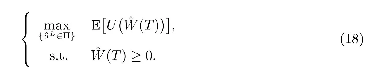
Since the auxiliary process(t) is self-financing, in order to ensure that the admissible investment strategy exists such that(T) ≥0, it is necessary and suきcient to assume that(0)=W(0)−G(0)≥0.

3.1.4 Solution of the auxiliary problem

where

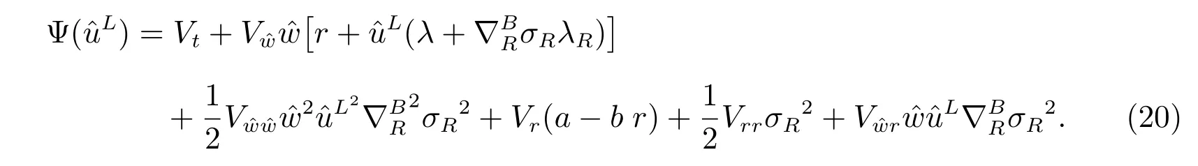
Vt, Vˆw, Vr, Vˆwˆw, Vrrand Vˆwrdenote the first and second order partial derivatives of V with respect to t,and r, respectively.

By the first order optimality condition, the optimal decision is expressed in terms of derivatives of the value function

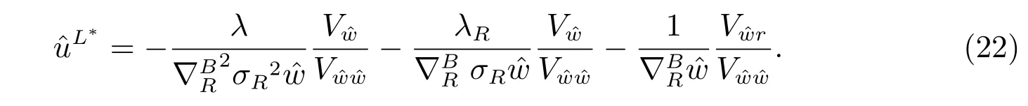
Substituting (22) into (19), we finally get the explicit form of the value function and the optimal investment strategy. The results are shown in the following theorem.

Theorem 1The optimal utility is given by

and the optimal investment strategy is given by

where

Proof See Appendix A.

3.1.5 Back to the original optimization problem

Based on the connection betweenLand uL, the optimal proportions for the original problem (12) are given by

In order to compare with the results in subsection 3.2,we denote the value function in subsection 3.1 by

3.2 Fund management with investment of an ordinary bond

Now we consider the performance of an ordinary zero coupon bond in the same pension plan and the same object. Here we abuse the notation and set the wealth process again denoted by W(t), but the portfolio consists of a bank account and an ordinary bond. The market is again complete. Similarly, the corresponding auxiliary process is defined by

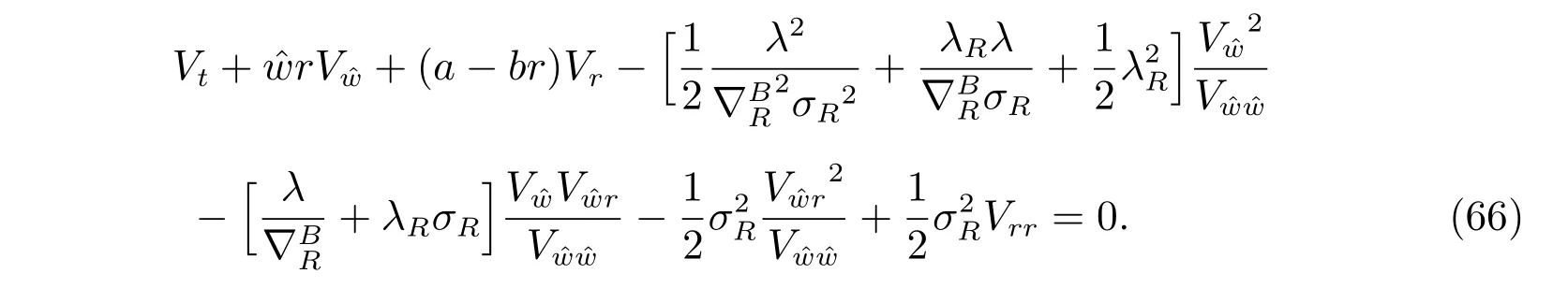
We have exactly the same objective function and the same optimization problem in subsections 3.1 and 3.2, except that the longevity bond is replaced by an ordinary bond. Analogously, denote V(t,r, ˆw) as the value function, the HJB equation is

By the first order optimality condition, we have the optimal strategy as the following

We can easily solve the above equation in a similar way. The results are described in the following theorem:

Theorem 2The optimal utility is given by

and the optimal investment strategy is given by

where

Proof The proof is similar to that of Theorem 1 so it is omitted here.

Back to the original problem by the connection between ˆuBand uB, we have

4 Optimal control during the decumulation phase

Now we consider the decumulation phase of the DC pension scheme. The problem is to find the optimal investment strategy from the retirement time 0 of a group of aきliates to a fixed time T (T ≤T0).

In the decumulation phase,see,for instance,Zimbidis and Pantelous[2],each member receives an accumulated amount,say,FTOT,at his or her retirement age. The total lump sum FTOTis separated into amount F1, which is converted to a pension annuity,and F2, which is converted to a whole life assurance with a death benefit.

According to Xiao et al[24]and Gao[25], we assume that the fund pays P(0) perpetuities to aきliates at time 0, then it pays P(t) perpetuities at time t for the coming years. Assume that P(t)is a deterministic and non-decreasing function of time t,whose growth rate depends on the rate of return on investments. This makes the contract more attractive to the aきliates. Thus we have

4.1 Fund management with investment of the longevity bond

4.1.1 The wealth process and optimization problem

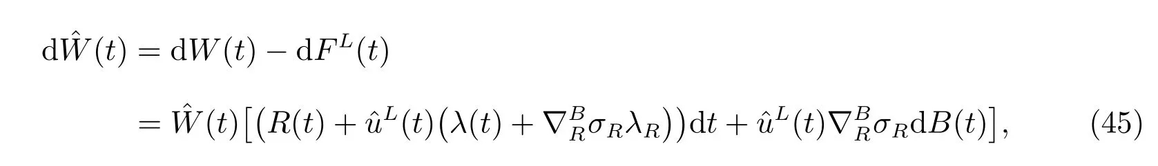
We consider the portfolio composed of a longevity bond and a riskless asset, in which case the market is complete. The wealth process associated with the strategy uL(t) invested into the longevity bond is given by

with an initial value W(0)=W0. The remainder(t)=1−uL(t)is the weight invested into the money market account. An investment strategy uL(t) is called admissible if it satisfies similar conditions as Definition 1. The set of all admissible controls is denoted by Π.

Following the work of Han and Hung[26], we define the expected lifetime utility at time t as the following

where Et{·} = E{·|Ft} is the conditional expection operator, Xτ= Wτ−Mτ, and M is a function of time t. Then the aim of the optimization problem is to maximize the function J over all admissible controls.

Here we abuse the death time of diあerent individuals and denote all of them by τ since they are i.i.d. variables. If the first death occurs after the terminal time T,our objective is to maximize the terminal wealth of the pension fund with a CRRA utility function. However, if it occurs before that, the pension fund should pay amount F2=Mτas death benefit to the beneficiaries at the death time τ, and then we would like to maximize the reminder fund, with the consideration of the second death, by using the method as same as the first step,and keep the cycle going until terminal time T.

According to the following facts that

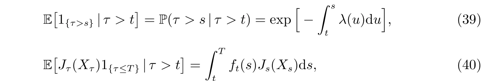
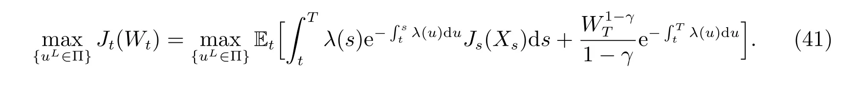
where ft(s) is given by (1), the initial optimization problem is transformed into the following problem with a certain time horizon T:

4.1.2 Construction of an auxiliary problem

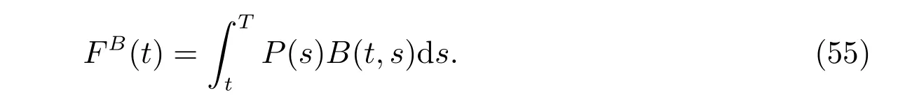
Now, we introduce an auxiliary process and transform problem (41) into a single one. Define the present value of the future annuity with the consideration of survival probability as follows

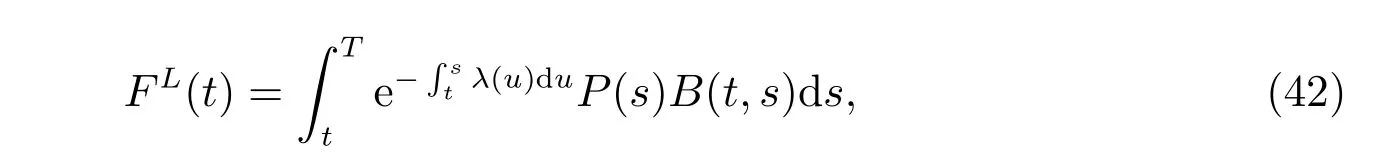
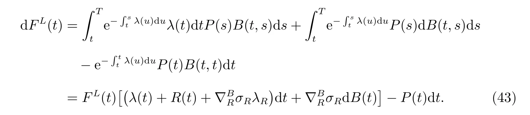
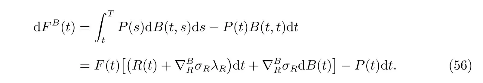
with the terminal condition FL(T)=0. B(t,s)is the present price of an ordinary bond with the terminal time s. Here B(t,s) can be regarded as the discounting factor. By diあerentiating, we have

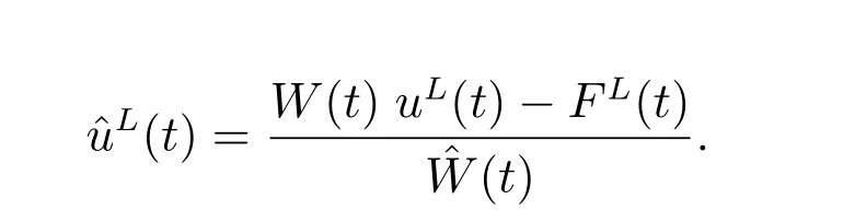
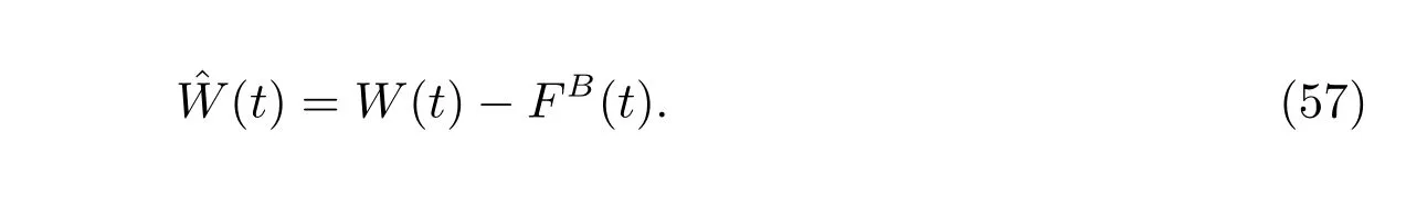
Then we define a corresponding auxiliary process as the following

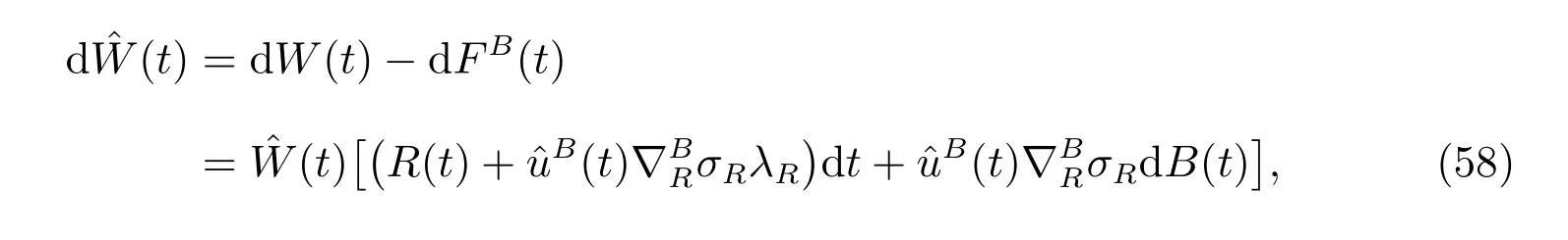
where

4.1.3 Solution of the auxiliary problem

Denote V(t,r, ˆw) as the value function of the auxiliary optimization problem (46).Thus the HJB equation is given by

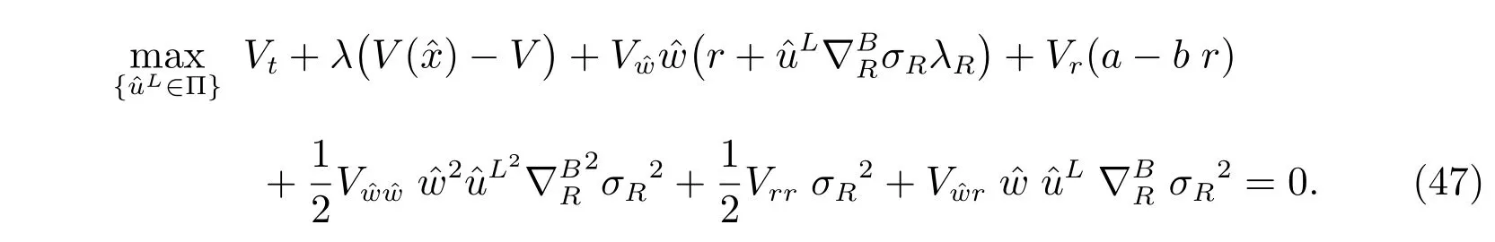
Taking derivative of the HJB equation with respect toLand considering the first order optimality condition, we obtain

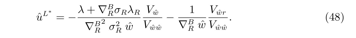
Substituting (48) into (47), we finally get the explicit form of V(t,r,) and the optimal policy, which is demonstrated in the following theorem.

Theorem 3Let c(t) be a deterministic function of time t. The optimal utility has the form of

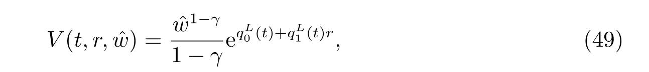
and the optimal investment strategy is given by

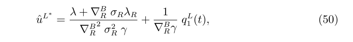
where

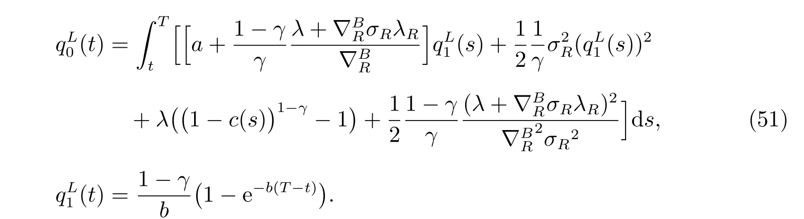
Proof See Appendix B.

4.1.4 Back to the original problem

Based on the connection between uLandL, we get the optimal proportions for the original problem

In order to compare with the results given by subsection 4.2, we denote the value function in subsection 4.1 by

4.2 Fund management with investment of an ordinary bond

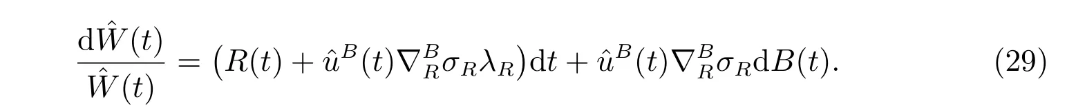
Now we consider the performance of an ordinary bond in a similar environment.We abuse the notation by denoting the wealth process again by W(t),but the portfolio consists of a bank account and an ordinary bond in this subsection, i.e.,

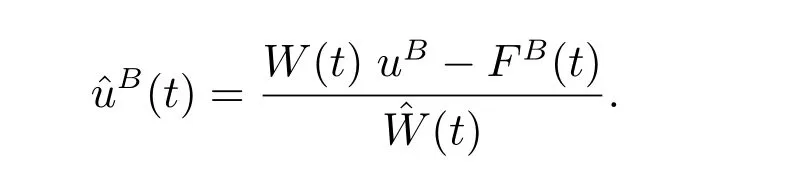
with the initial condition W(0) = W0.(t) and uB(t) are proportions invested into the riskless asset and the ordinary bond, respectively. Similarly, a fictitious asset is defined by

By diあerentiating, we obtain that

Then we define the corresponding auxiliary process similar to that of subsection 4.1:

So we have

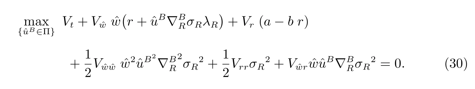
where

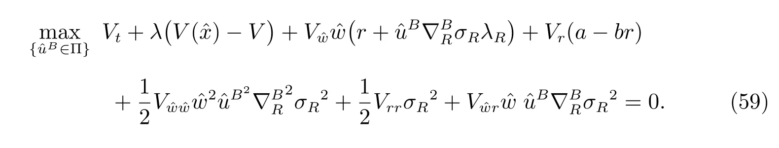
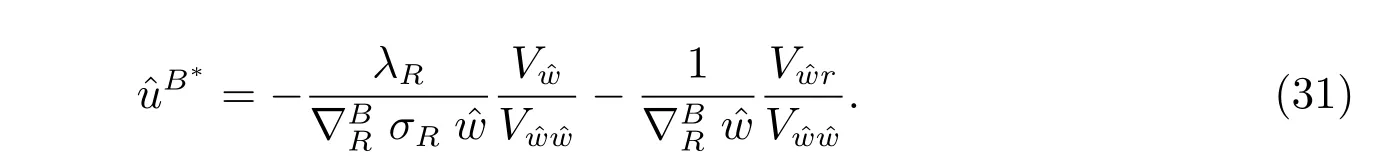
The optimal policy is determined by the first order optimality condition with respect to

We can easily solve the above equation in the same way. The results are described in the following theorem.

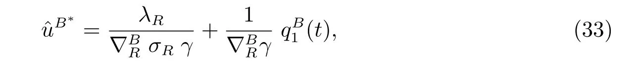
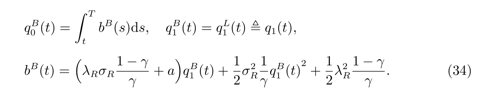
Theorem 4Let c(t) be a deterministic function of time t. The optimal utility has the form of

and the optimal investment strategy is given by

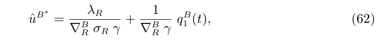
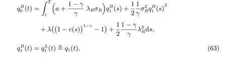
Proof The proof is similar to that of Theorem 3 so we omit it here.

When we back to the original problem by the connection between uB(t)andB(t),we have

5 Sensitivity analysis, comparative study and conclusion

In this section, we first make some sensitivity analyses to show the relationship between the optimal investment strategy and some parameters in subsection 3.1 and subsection 4.1,respectively. Then,in order to show the impact of the longevity bond on the optimal expected utility function in both the accumulation and the decumulation phase, a comparative study between subsection 3.1 and subsection 3.2, and also a comparative study between subsection 4.1 and subsection 4.2 are given in the following subsection.

5.1 Sensitivity analyses

Unless otherwise stated, the values of parameters are given as follows: λ = 0.2,σR=0.5, b=0.1,=−1, λR=−1, C0=1, W0=1, t=0, T =30 and γ =0.5.

From Figure 1 to Figure 4,we investigate the relationships between the investment decision and parameters in subsection 3.1. Figure 1 gives the relationship between the volatility and the optimal weight of the longevity bond. With suitable parameters chosen, the pension trustee takes a short position on the longevity bond. It is easy to conclude that the absolute value of the optimal weight decreasing with the absolute value of the volatility increasing. Since the trustee faces more risk with higher absolute volatility, the absolute optimal decision may decrease to avoid investment risk.

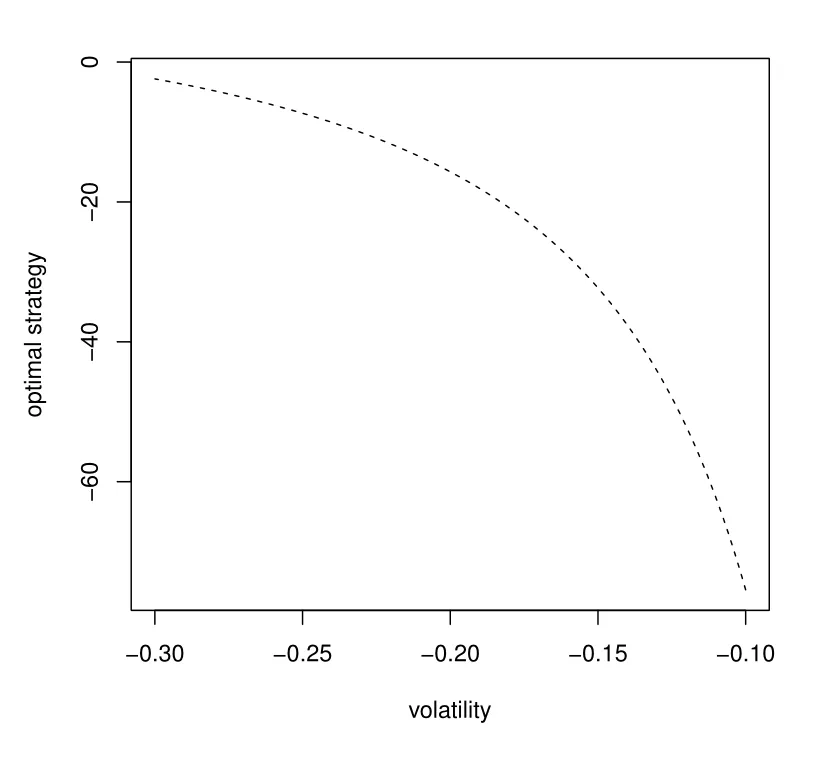
Figure 1: Impact of σR in the first phase

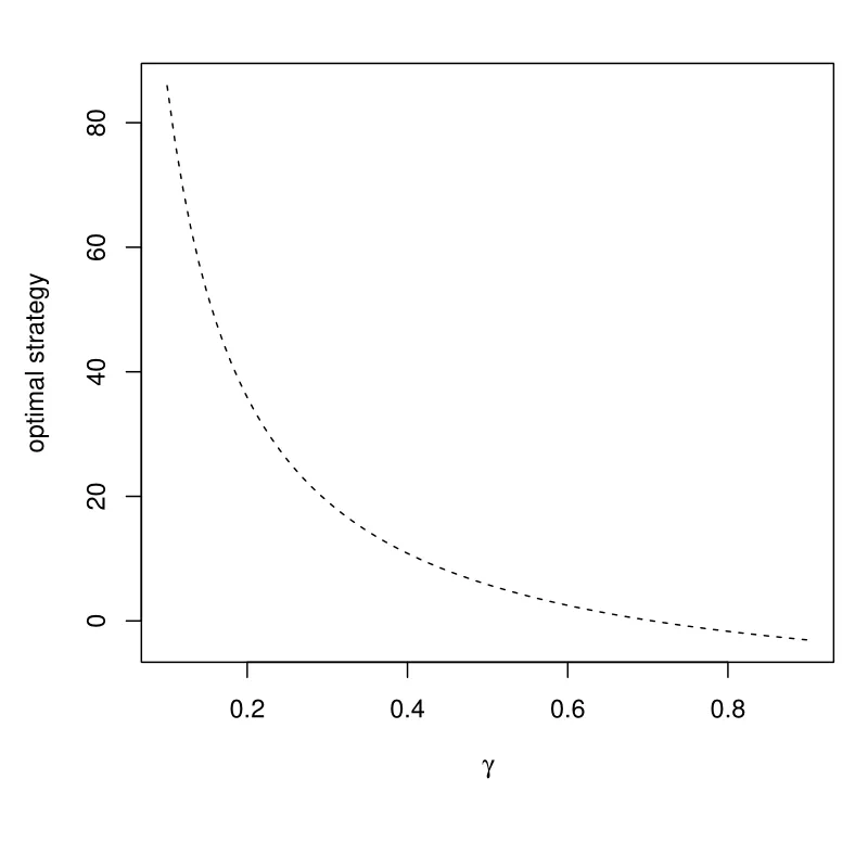
Figure 2: Impact of γ in the first phase

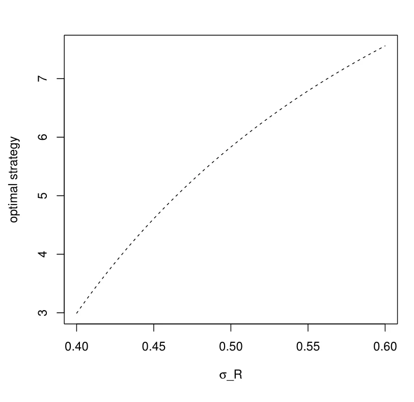
Figure 3: Impact of σR in the first phase

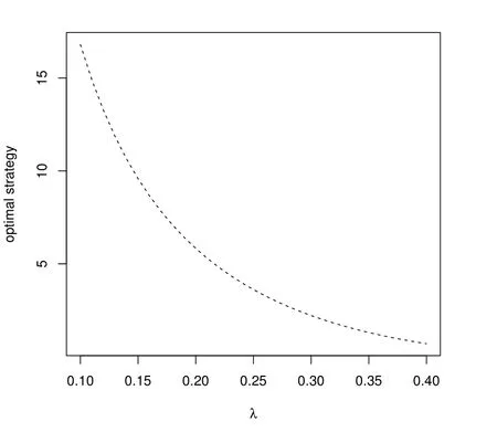
Figure 4: Impact of λ in the first phase

Figure 2 shows the relationship between the measure of the relative risk aversion in the CRRA utility function and the portfolio chosen. It seems that the optimal investment in the risky asset decreases when the investor tends to be more risk-averse.

Figure 3 investigates the influence of the volatility of the interest rate, which reflects shakes in return of the riskless asset. With the uncertainty in the riskless asset increasing, the pension manager holds a smaller proportion of the bank account in his or her portfolio, thus the proportion of the longevity bond increases.

Figure 4 considers the influence of the hazard rate. The trustee faces higher longevity risk with lower hazard rate. The figure shows that the optimal weight of the longevity bond increases when the mortality rate decreases. Thus, under suitable parameters chosen,it is reasonable to conclude that the longevity bond do have significant advantage to hedge longevity risk in the accumulation phase of a DC pension scheme.

From Figure 5 to Figure 8,we investigate the relationships between the investment decision and the parameters in subsection 4.1. With suitable parameters, Figure 5 shows that the pension manager takes a short position on the longevity bond, which is similar to the phenomenon in the accumulation phase. As shown in the figure, the absolute value of optimal investment in the longevity bond decreases with the absolute value of the volatility ∇σRincreasing. A reasonable explanation of this phenomenon is that the trustee faces higher risk with higher volatility, thus he or she may adjust the optimal weight of the risky asset in order to avoid investment risk.

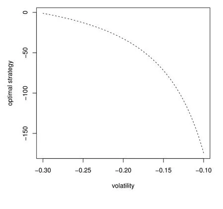
Figure 5: Impact of σR in the second phase

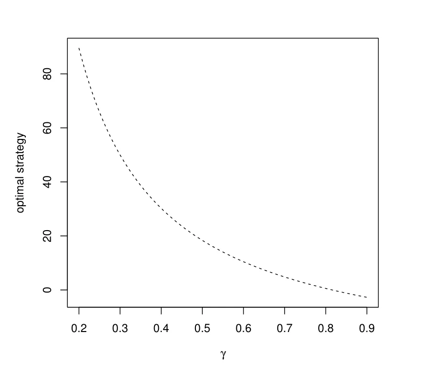
Figure 6: Impact of γ in the second phase

To investigate the relationship between the measure of the relative risk aversion γ and the optimal portfolio in the decumulation phase, Figure 6 shows that the weight of the longevity bond decreases when the pension trustee tends to be more risk-averse,which coincides with the result in the accumulation phase.

Figure 7 considers the influence of σR, which is the volatility of the interest rate.With fixed γ, the portfolio has a smaller proportion of the riskless asset with a higher uncertainty in the bank account. Thus, the remainder, proportion of the longevity bond increases.

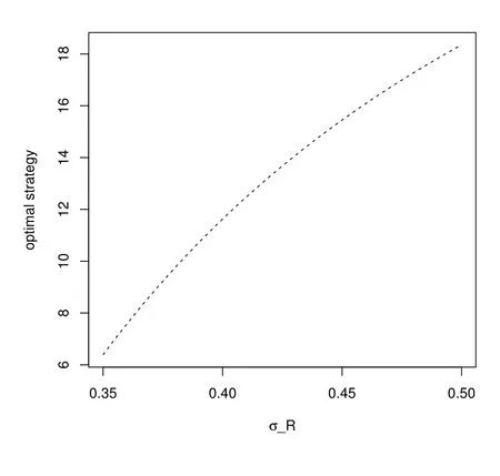
Figure 7: Impact of σR in the second phase

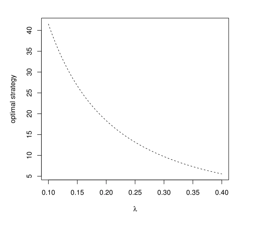
Figure 8: Impact of λ in the second phase

As it has illustrated in the accumulation phase, the pension manager faces higher longevity risk with lower mortality rate. In order to investigate the impact of the hazard rate, Figure 8 gives that the proportion of the longevity bond increases with a decreasing mortality rate. Thus, with the consideration of Figure 4, it is reasonable to say that the longevity bond can hedge longevity risk in our model, during both accumulation and decumulation phase.

5.2 Comparative study

This subsection considers comparative studies between the results in subsections 3.1 and 3.2, and results between subsections 4.1 and 4.2. Let σR= 2.05, b = 0.5,= −1, λR= −2, C0= 1, W0= 1, t = 0, T = 30 and γ = 0.5. First we compare(23) and (32) and have the following theorem.

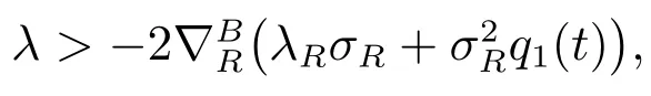
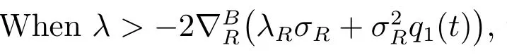
Next we make a comparison between subsections 4.1 and 4.2. By comparing (49)and (61), we have the following theorem.

If we calculate the ratio between VLand VBat the initial time as

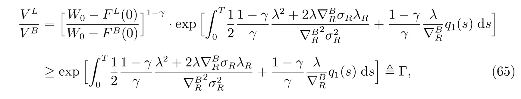
it is easy to conclude by Figure 10 that Γ ≥1 and it almost has an exponential growth with the increasing rate of mortality, and so is VL/VB.

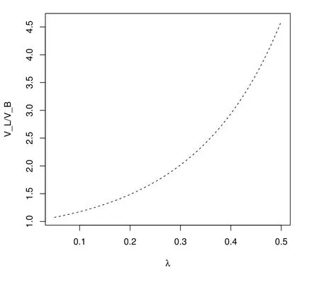
Figure 9: Impact of λ to the ratio

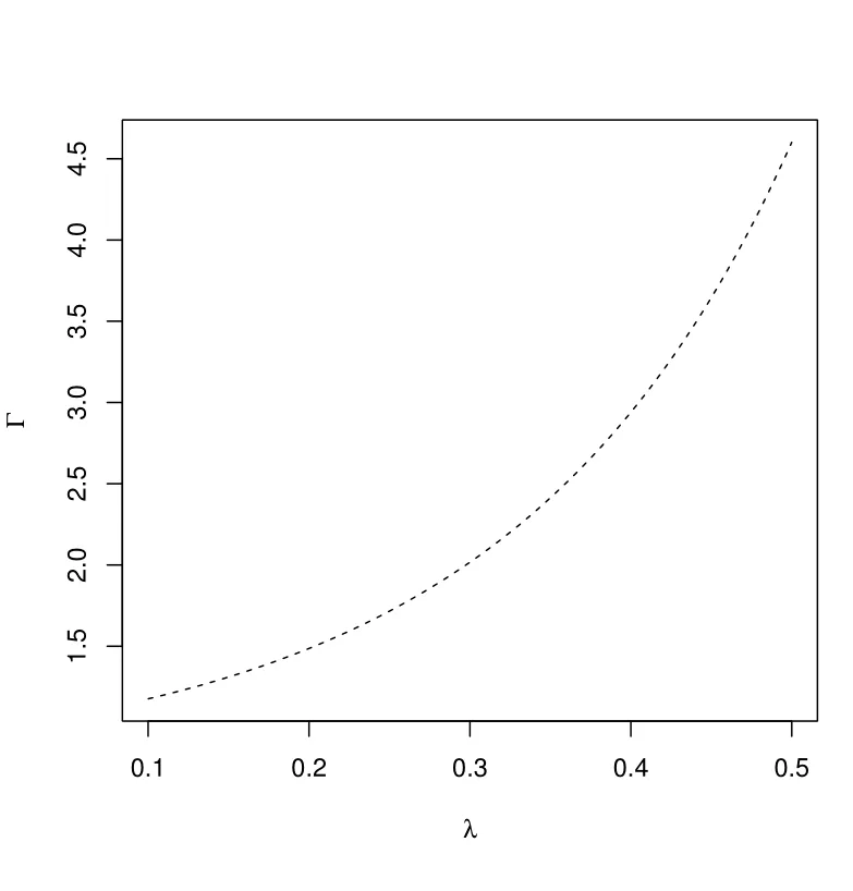
Figure 10: Impact of λ to Γ

5.3 Conclusion

This paper investigates, by the dynamic programming approach, two optimal investment problems for a DC pension fund, in a stochastic interest rate and uncertain life time framework. For both problems, the objectives are to determine the optimal investment strategy maximizing the terminal wealth with a CRRA utility function. Explicit solutions are derived from the HJB equations,which can be solved via two ODEs,respectively. We find that under some rational assumptions, a longevity bond do have significant advantages to improve the investment eきciency in both accumulation and decumulation phases in such a pension scheme.

Appendix A

The proof of Theorem 1.

Substituting (22) into the HJB equation (19), we get

The structure of the HJB equation suggests an exponential solution of the following form

with the terminal conditions(T)=(T)=0.

By diあerentiating, we have

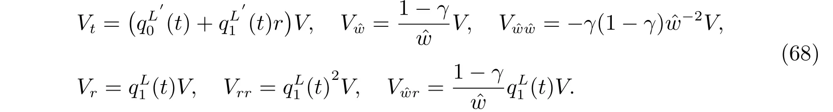
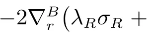
Substituting (68) into (66), and arranging it by order of r, we have

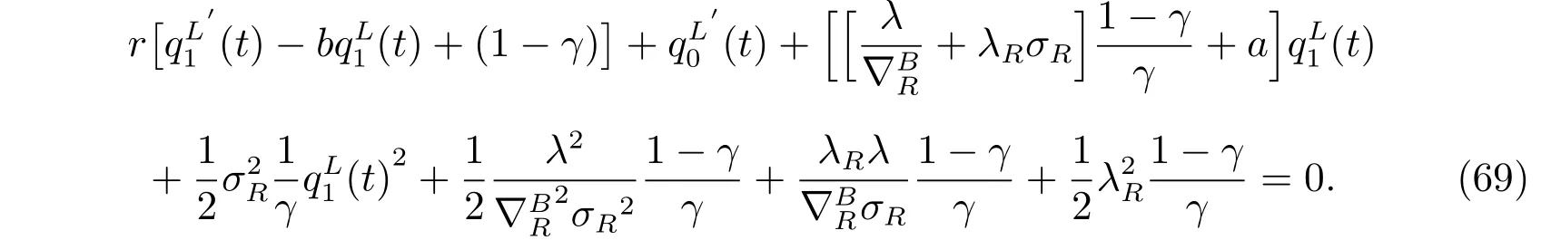
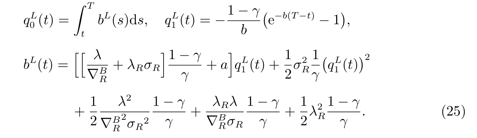
The above equation holds for every r. With the terminal conditions,it is equivalent to the following two equation systems

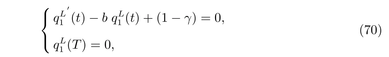
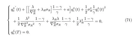
The results hold by solving (70) and (71). The optimal investment strategy is obtained by substituting the derivatives of the value function into the first order optimality condition in (22).

Appendix B

The proof of Theorem 3.

Substituting (48) into the HJB equation (47), we get

The structure of the HJB equation suggests an exponential solution of the form

Diあerentiating it, we get

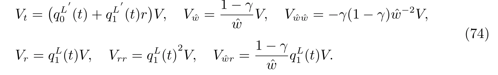
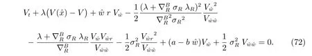
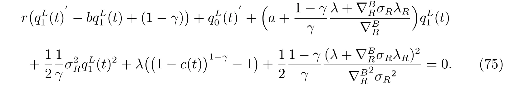
After substituting (74) into (72), and arranging it by order of r, we get

We set M(t)=c(t)ˆW(t) in the above equation, where c(t) is a deterministic function of t, i.e., the death benefit is a specific proportion of the total fund.

Since the above equation holds for every r, it is equivalent to the following two ODEs

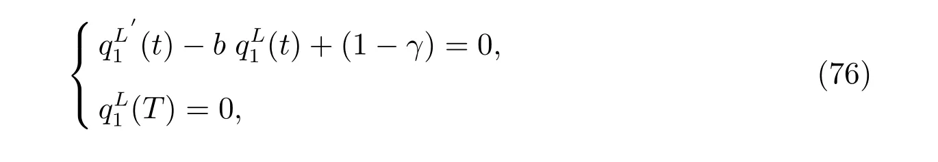
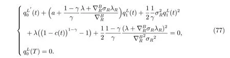
The result holds by solving (76) and (77). By substituting the derivatives of the value function into the first order optimality condition (48), the optimal investment weight is obtained.