基于指数模型的R = P(Y ＜X ＜Z)统计推断

程从华

（肇庆学院 数学与统计学院，广东 肇庆 526061）

1 Introduction

Let X,Y,Z be the three random variables,the stress-strength model of the types R = P(Y ＜X) or R = P(Y ＜X ＜Z)have extensive applications in various subareas of engineering，psychology，clinical trials and so on，since these models provide general measure of the genetics，difference between or among populations. One is referred to the monograph by Kotz，Lumelskii and Pensky[1]and references therein.In context of medicine and genetics，a popular topic is the analysis of the discriminatory accuracy of a diagnostic test or marker in distinguishing between diseased and nondiseased individuals，through the receiver-operating characteristic (ROC) curves. Estimation of R for the case of Burr Type X distributions for X and Y was discussed by Ahmad et al.[2]，Surles and Padgett[3-4]and Raqab et al.[5]

One can also find many interesting practical examples in Kotz et al.[1]Some studies are concerned about the estimation of R. Dreiseitl, Ohno Machado and Binder[6]suggest estimating R by three-sample U-statistics. Waegeman，De Baets and Boullart[7]proposed a fast algorithm for the computation of P(Y ＜X ＜Z)and its variance using the existing U-statistics methods. Ivshin[8]investigates the MLE and UMVUE of θ when X，Y and Z are either uniform or exponential r.v.s with unknown location parameters.More reference about statistical inference of P(Y ＜X ＜Z)or P(Y ＜X)can be seen in Wang et al.[9]，Chen et al.[10]，Amay et al.[11]，Baker et al.[12]and Jia et al.[3]In this paper，our methods provide easier and better alternative tools to do inference of R.

In this article，different point estimators of R are derived，MLE and Bayesian estimators with mean squared error loss functions.Based on the MLE，we can obtain the exact confidence interval of R.Also，we obtain the approximate confidence interval for R by using the approximate normal property of the MLE of R.In addition，based on the Bayesian estimator，we obtained the Bayesian credible interval of R.Different methods have been compared by using Monte Carlo simulations.

The rest of the paper is organized as follows.In section 2，the MLE and Bayesian estimation of R are presented and the explicit expression of R is also derived. In section 3，different interval estimators of R are presented，including exact，approximate，and Bayesian credible intervals. Some numerical experiments and some discussions are presented in section 4.

2 Point estimations of R

2.1 Maximum likelihood estimation of R

A random variable(r.v.)X is said to have exponential distribution if its probability density function (pdf)is given by

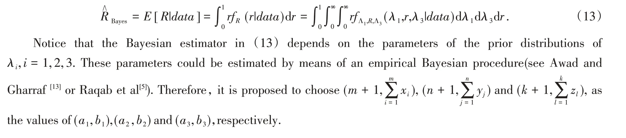
The cumulative distribution function is

where λ ＞0,x ＞0.An exponential distribution will be denoted by ε(λ).

Let X be the strength of a system，Y and Z be the stress acting on it. Assume that X ～ε(λ1), Y ～ε(λ2),Z ～ε(λ3)are independent.Therefore，the reliability of the system will be

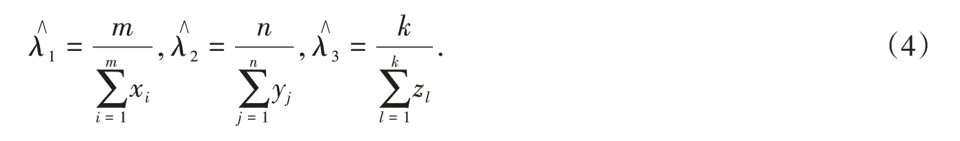
To compute MLE of R，we need the computation of the MLE of λ1,λ2,λ3. Suppose X1,X2,…,Xmis a random sample from ε(λ1)，Y1,Y2,…,Ynis a sample from ε(λ2)and Z1,Z2,…,Zkis a sample from ε(λ3). The likelihood function for the observed sample is

The ln likelihood function is

To obtain the MLEs of λ1,λ2and λ3，we can maximize L(λ1,λ2,λ3)directly with respect to λ1,λ2and λ3.Differentiating（3）with respect to λ1,λ2and λ3，respectively and equating to zero，we obtain the following equations，

Then，the MLE of λ1,λ2,λ3are

Based on the invariance of maximum likelihood estimation，then the MLE of R becomes

2.2 Bayesian estimation of R

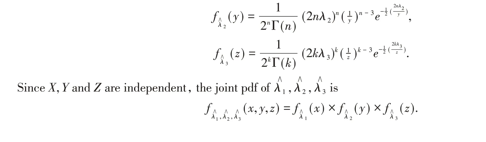
In this subsection，we obtain the Bayesian estimation of R under the assumption that the parameters λi,i =1,2,3 are independent random variables. It is assumed that λi,i = 1,2,3 have independent gamma priors with the pdfs

with the parameters λi～Gamma(ai,bi),i = 1,2,3.The posterior pdfs of λiare as follows:

Since the priors of λi,i = 1,2,3are independent，using（7）-（9），the joint posterior pdf of(Λ1,Λ2,Λ3)is

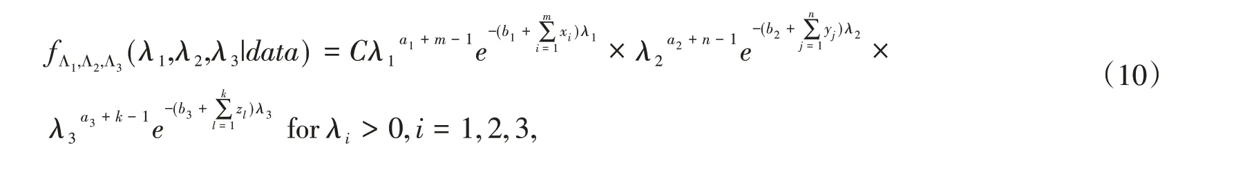
where

Applying the probability density formula of random variable function，the joint posterior pdf of(Λ1,R,Λ3)is

It is that

Therefore，the posterior marginal distribution of R is

Now，consider the following loss function:

It is well known that Bayes estimates with respect to the above loss function is the expectation of the posterior distribution.The Bayes estimate of R under squared error loss cannot be computed analytically.

3 Interval estimation of R

3.1 Exact confidence interval

Based on the Subsection 2.1，it is clear that

It is easy to see that

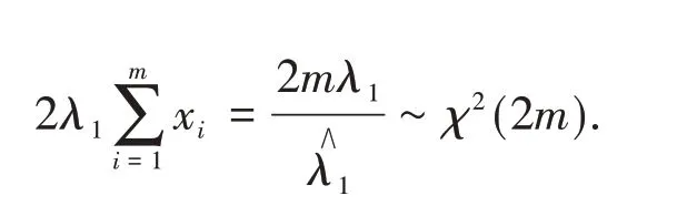
Similarly，we have

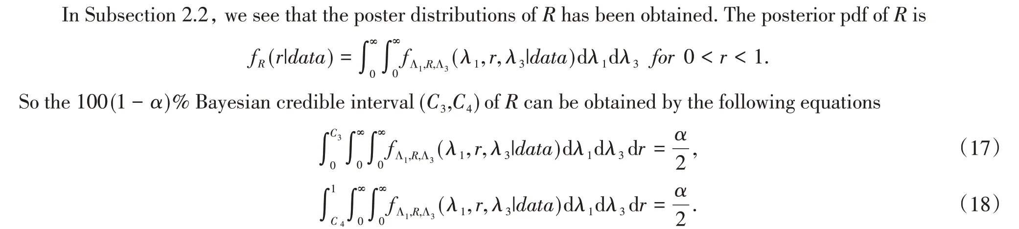
3.2 Bayesian credible interval

3.3 Approximate confidence interval

We denote the Fisher information matrix of θ =(λ1,λ2,λ3)as I(θ)，where I(θ) =[Iij]i,j=1,2,3is

It is easy to see that

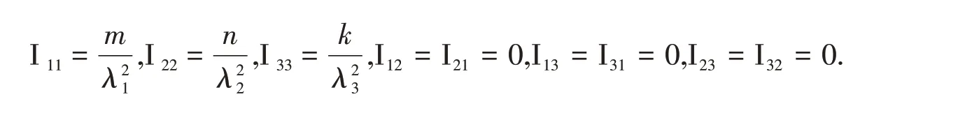
Now the asymptotic covariance matrix[A]i,j=1,2,3for the MLEs of λ1,λ2and λ3is obtained by inverting the Fisher matrix，ie.A=[I(θ)]-1

where Z(1-γ/2))if the 100(1- γ/2)%)the quantile of the standard normal distribution.

4 Simulations and discussions

In this section，we present some results based on Monte Carlo simulations to compare the performance of the different point estimators and interval estimations for different sample sizes and different parameter values.

（1）The point estimations of R，that is，the MLE and Bayesian estimation.

（2）The interval estimations of R，that is，the exact，the approximate and the Bayesian credible intervals.

In all cases，we consider the following small samples，(m,n,k) =(10,10,10), (10,15,15), (10,10,20),(10,20,30),and we take λ1= 1.5,2.0,3.0,λ2= 1.5,2.0,3.0,3.5,and λ2= 2.0,2.5,3.0,4.0,respectively.All the results are based on 10000 replications.

Case（i）

From the sample，we estimate λi,i = 1,2,3 using（4）. Then we obtain the MLE of R using（5）. In addition，we obtain the Bayesian estimation using (13). We report the average biases and mean squared errors (MSEs) in Table1 over 10000 replications.Some of the points are quite clear from Table 1.

（1）Even for small sample sizes，the performance of the MLEs and Bayesian estimations are quite satisfactory in terms of biases and MSEs. For example，when(λ1,λ2,λ3)=(1.5,1.5,2) and(m,n,k) =(10,15,15) the biases and MSEs for above three estimation of R are 0.002 6，-0.001 1 and 0.001 7，0.000 4，respectively.

（2）It is observed that when n,k increase，the MSEs decrease. This verifies the consistency property of the MLE and Bayesian estimation of R. For example，when (n, k) increase to(20,30)，the corresponding above values decreased to 0.002 6，0.004 4 and 0.001 4，0.001 4，respectively.

（3）For fixed n，as m increases，the MSEs decrease. For fixed m，as n increases，the MSEs decrease as expected.

Case（ii）

Now let us consider the exact，approximate interval estimation and Bayesian credible interval for R.In this experiment，we report the confidence intervals of R and coverage probabilities for all sample sizes and parameter values.

From Table 2，we can see that

Table 1 Biases and MSEs of point estimations of parameters

（1）It is observed that the average length of exact confidence interval is shorter than that of approximate confidence interval but is longer than that of Bayesian credible interval. For example，when(m,n,k) =(10,15,15) and(λ1,λ2,λ3)=(1.5,3.0,3.0)，the lengths of three confidence interval are 0.175 5，0.282 4 and 0.126 9，respectively.

（2）The average lengths of all intervals decrease as m or n increases.For example，for Bayesian method，when(λ1,λ2,λ3)=(3.0,1.5,1.5),the lengths of the confidence intervals corresponding to four combinations of n and m,(10,10,10),(10,15,15),(10,10,20),(10,20,30)are 0.147 0，0.160 6，0.176 4 and 0.157 7，respectively.

（3）It is observed that the coverage probabilities of the methods in this article are all close to the nominal level.It shows that these methods are applicable.

（4）Among the different confidence intervals，Bayesian credible interval has the shortest confidence length.

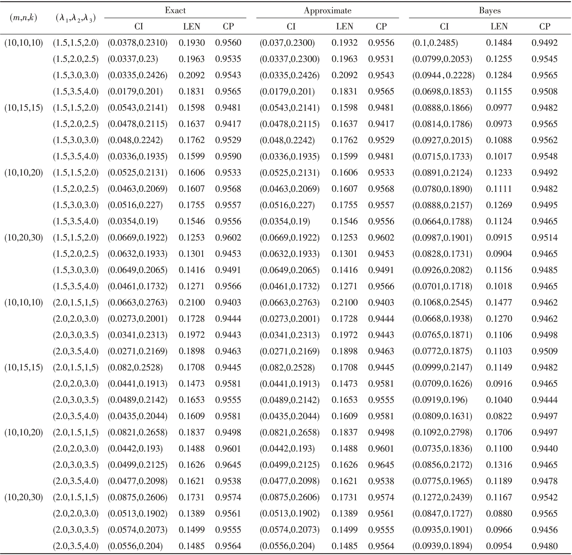
Table 2 Confidence intervals for exact，approximate and Bayesian credible intervals