随机矩阵特征值新盖尔型包含集(英)

(A)=trace(A)+(n −1)(A)−1,

|µ−0.2255|≤1.6380.

|µ+0.2008|≤1.3461.

|µ|≤0.5846.

1 Introduction

As it is well known,stochastic matrices and the eigenvalue localization of stochastic matrices play the central role in many application fields such as birth and death processes, computer aided geometric design and Markov chain, see [1-6]. An nonnegative matrix A=(aij)∈Rn×nis called a row stochastic matrix(or simply stochastic matrix)if for each i ∈N ={1,2,··· ,n},that is,the sum of each row is 1. Since the row sum condition can be written as Ae=1e,we find that 1 is an eigenvalue of A with a corresponding eigenvector e=[1,1,··· ,1]T.It follows from the Perron-Frobenius theorem[7]that |λ| ≤1,λ ∈σ(A). In fact, 1 is a dominant eigenvalue for A. Furthermore, η is called a subdominant eigenvalue of a stochastic matrix if η is the second-largest modulus after 1[8,9].

In 2011,Cvetkovi´c et al[10]discovered the following region including all eigenvalues different from 1 of a stochastic matrix A by refining the Gersgorin circle[11]of A.

Theorem 1[10]Let A = (aij) ∈Rn×nbe a stochastic matrix, and let si, i = 1,2,··· ,n be the minimal element among the off-diagonal entries of the ith column of A.Taking γ(A)=maxi∈N(aii−si), if λ ̸=1 is an eigenvalue of A, then

However, although (1) of Theorem 1 provides a circle with the center γ(A) and radius r(A) to localize the eigenvalue λ different from 1, it is not effective when A is stochastic, and aii=si=0, for each i ∈N.

Recently, in order to conquer this drawback, Li and Li[12]obtained the following modified region including all eigenvalues different from 1.

Theorem 2[12]Let A = (aij) ∈Rn×nbe a stochastic matrix, and let Si, i = 1,2,··· ,n be the maximal element among the off-diagonal entries of the ith column of A. Taking(A)=maxi∈N(Si−aii), if λ ̸=1 is an eigenvalue of A, then

Note that (2) of Theorem 2 provides a circle with the center −(A) and radius(A).

In general, the circle of Theorem 1 and Theorem 2 can be large when n is large. It is very interesting how to provide a more sharper Gersgorin circle than those in[10,12].

In this paper,we will continue to investigate the eigenvalue localization for stochastic matrices and present a new and simple Gersgorin circle set that consists of one disk.Moreover, an algorithm is obtained to estimate an upper bound for the modulus of subdominant eigenvalues of a positive stochastic matrix. Numerical examples are also given to show that our results are more effective than those in [10,12].

2 A new eigenvalue localization for stochastic matrices

Here matrices A with constant row or column sum are considered,that is,Ae=λe or ATe = λe for some λ ∈R. Obviously, λ is an eigenvalue of A, when λ = 1, it is stochastic.

To obtain a new set including all eigenvalues different from 1 of a stochastic matrix,we start with the following propositions.

Proposition 1[10]Let A=(aij)∈Rn×nbe such that ATe=λe, for any d=[d1,d2,··· ,dn]T∈Rn×n, let µ∈σ(A){λ} . Then −µ is also an eigenvalue of the matrix

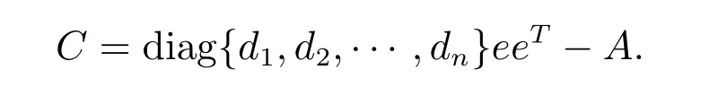
Applying this result to AT, we have:

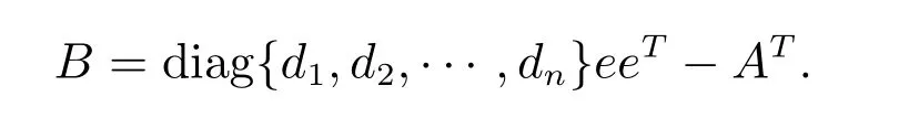
Proposition 2[10]Let A = (aij) ∈Rn×nbe such that Ae = λe, for any d = [d1,d2,··· ,dn]T∈Rn×n, let µ∈σ(A){λ}. Then −µ is also an eigenvalue of the matrix

It is easy to see that the best choice of each diin Proposition 1 and Proposition 2 should minimize the radius of the ith Gersgorin row circle of C and B. In particular,we present the following choice for an nonnegative matrix

which not only leads to a reduction of the radii of the Gersgorin circles,but also localizes all eigenvalues in one circle.

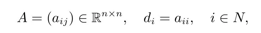
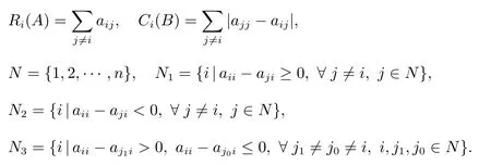
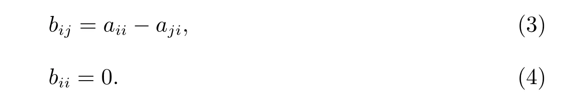
Firstly, let us introduce some notations. For an nonnegative matrix A = (aij) ∈Rn×n, which is a stochastic matrix, and B = diag{d1,d2,··· ,dn}eeT−AT, where di=aii, define, for i=1,2,··· ,n,

The main result of this paper is the following theorem.

Theorem 3Let A=(aij)∈Rn×nbe a stochastic matrix,taking di=aii, i ∈N,if λ ̸=1 is an eigenvalue of A, then:

(I) If N1=N, then |λ|≤¯r(A)=trace(A)−1;

(II) If N2=N, then |λ|≤¯r(A)=1 −trace(A);

(III) If N3̸=∅, then

Proof Since di=aii, i ∈N,and B =diag{d1,d2,··· ,dn}eeT−AT,we have that for any i ∈N, and j ̸=i,

如自学习《鸦片战争》时，鸦片战争打开了我国的大门，为我国带来了侵略、伤害。但同时进了我国自然经济的解题，让我过从封闭天国转变出来，开始面向社会。它也成为了我国现代史的开端，所以学生不能够从单一的角度去认识和学习它，而要从辩证的角度去看待它。

Firstly, we consider the following two special cases (I) and (II). From (3), we have:(I) If N1=N, for each i ∈N, j ̸=i, it has

so, by (4), Proposition 2 and Gersgorin circle theorem, we have

(II) If N2=N, similarly, for each i ∈N, j ̸=i,

then

In general, that is, the following case (III), we have:

(III) If N3̸=∅, so, by (4), Proposition 2 and Gersgorin circle theorem, we obtain

The proof is completed.

Remark 1Note that the special cases (5) and (6) of Theorem 3 provide circles with the center 0 and radius equal to trace(A)−1 and 1 −trace(A), respectively. The two bounds are not sharper than (1) of Theorem 1 and (2) of Theorem 2. However,more generally, for case (III), we have

Remark 21) Consider the following matrix, it illustrates that the bound provided by Theorem 3 is sharp. Take the matrix

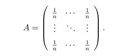
Then

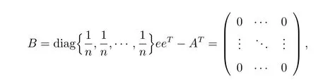
by Theorem 3, |λ|≤0. In fact, the eigenvalues of A different from 1 are 0.2) Furthermore, consider the following matrix

By Theorem 1, for any µ ∈σ(A)1, we have |µ−0.3096| ≤1.1234. By Theorem 2,we have |µ+0.1273| ≤0.6242. By Theorem 3, we have µ| ≤0.3776. These regions are shown in Figure 1. It is easy to see that the region in Theorem 3 localizing all eigenvalues different from 1 of A is better than those in Theorem 1 and Theorem 2.

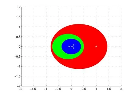
Figure 1 The region |µ|≤0.3776 is represented by the innermost circle

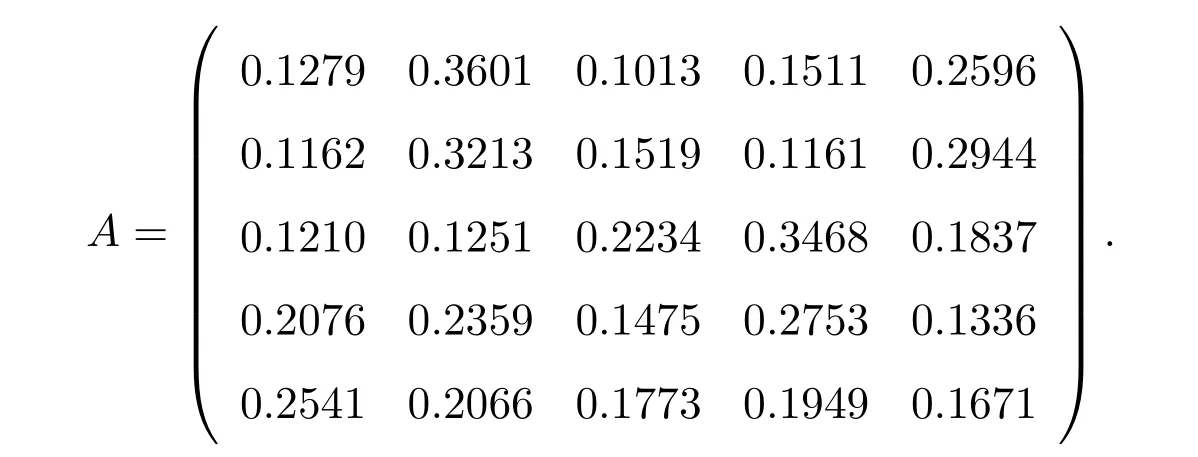
In order to further compare obtained results, we consider the following stochastic matrix generated by the Matlab code

By Theorem 1, for any µ∈σ(A)1, we have

|µ−0.2255|≤1.6380.

By Theorem 2, we have

|µ+0.2008|≤1.3461.

By Theorem 3, we have

|µ|≤0.5846.

These regions are shown in Figure 2, obviously,our result is better than those got from Theorem 1 and Theorem 2 in some cases.

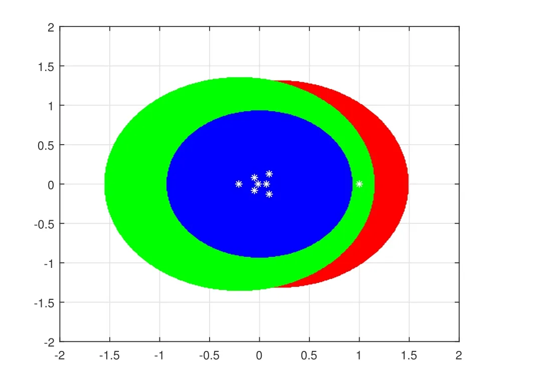
Figure 2 The region |µ|≤0.5846 is represented by the innermost circle

3 Comparison of the subdominant eigenvalue of stochastic matries

Note that if A is stochastic, then Amis also stochastic for any positive integer m.Cvetkovi´c et al[10], applied Theorem 1 to obtain

and proved that the sequences {γm(A)} and rm(A) all converge to 0, where the value γm(A)=γ(Am).

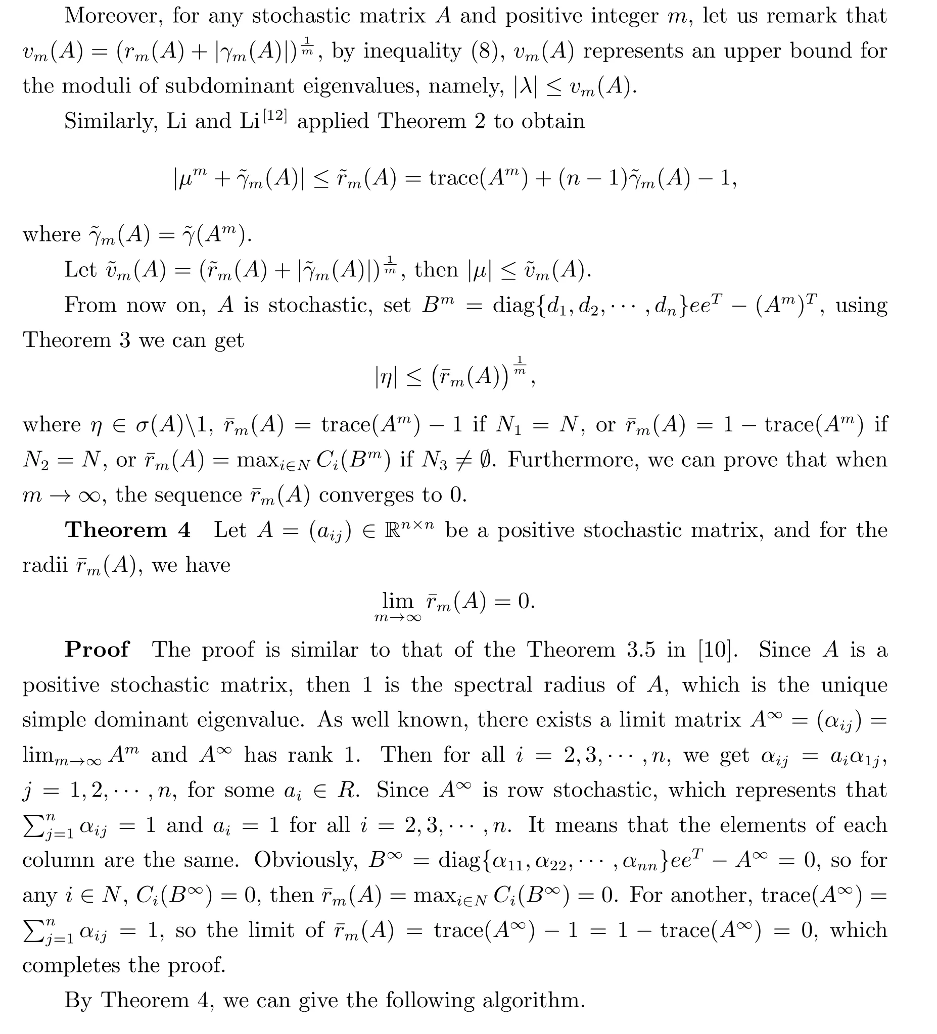
Algorithm 1Given a positive stochastic matrix A=(aij)∈Rn×nand a positive integer T, for t=1, do the following:

1) Set m=2t−1;

2) Compute Bm=diag{d1,d2,··· ,dn}eeT−(Am)T;

3) If N1=N, computem(A)=trace(Am)−1;

4) If N2=N, computem(A)=1 −trace(Am);

5) If N3̸=∅, computem(A)=maxi∈NCi(Bm);

6) Set A=A×A and t=t+1. If t>T, output r, stop, otherwise, go to 1).

Example 1Stochastic matrices A1, A2are the same as in [10,12].

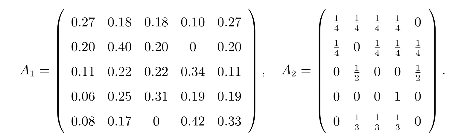
Using Matlab, we can compute vm(A),m(A) andm(A), see Table 1 and Table 2,respectively.

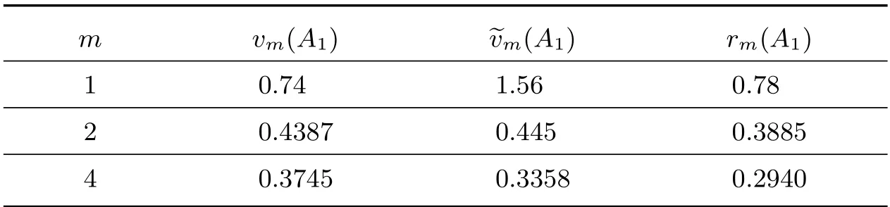
Table 1 The value for A1 when m=2t, t=0,1,2

By Matlab computations, the eigenvalues of A1are 0.1634,0.2094±0.1109i, and 0.1732.

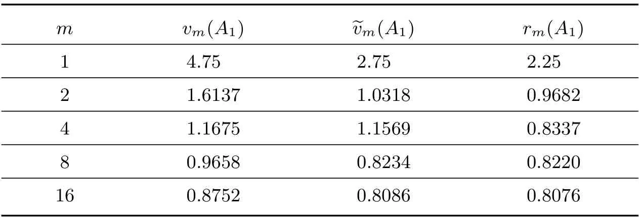
Table 2 The values for A2 when m=2t, t=0,1,2,3,4

By Matlab computations, the eigenvalues of A2are 0.7934,−0.3683±0.0088i, and 0.1936. We can observe that Theorem 3 is better than those in [10,12].

Example 2

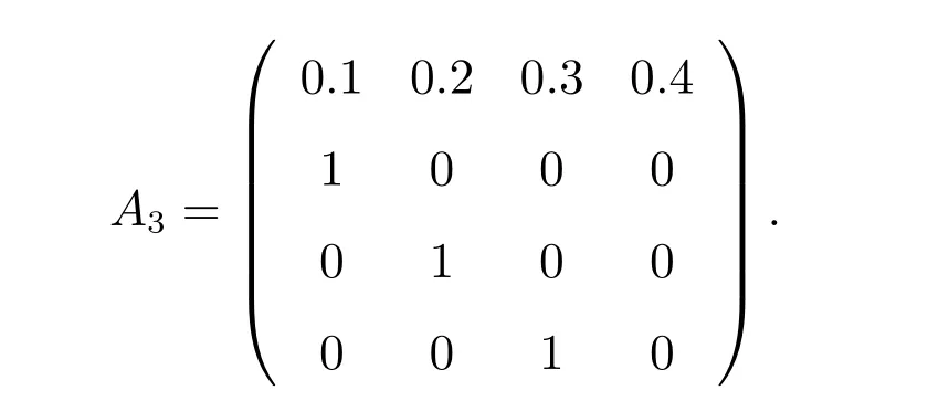
Matrix A3is the example in [10] with xi= i/10, i ∈{1,2,3,4}. By computations,vm(A3),m(A3) andm(A3) are shown in Table 3.

Table 3 The values of vm(A3), m(A3) and m(A3)

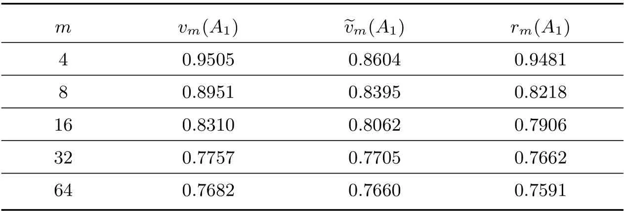
Table 3 The values of vm(A3), m(A3) and m(A3)

m vm(A1) ～vm(A1) rm(A1)4 0.9505 0.8604 0.9481 8 0.8951 0.8395 0.8218 16 0.8310 0.8062 0.7906 32 0.7757 0.7705 0.7662 64 0.7682 0.7660 0.7591

By Matlab computations, the second-largest eigenvalue of A3is 0.7513. It is not difficult to see from this example that our bound performs better than that in [10,12].