
Quantum algorithm for a set of quantum 2SAT problems∗
2021-03-11 08:31YanglinHu胡杨林ZhelunZhang张哲伦andBiaoWu吴飙
Chinese Physics B 2021年2期
关键词:胡杨林
Yanglin Hu(胡杨林), Zhelun Zhang(张哲伦), and Biao Wu(吴飙),2,3,†
1International Center for Quantum Materials,School of Physics,Peking University,Beijing 100871,China
2Wilczek Quantum Center,School of Physics and Astronomy,Shanghai Jiao Tong University,Shanghai 200240,China
3Collaborative Innovation Center of Quantum Matter,Beijing 100871,China
Keywords: adiabatic quantum computation,quantum Hamiltonian algorithm,quantum 2SAT problem
1. Introduction
In 1990s, several quantum algorithms such as Shor’s algorithm for factorization and Grover’s algorithm for search[1]were found to have a lower time complexity than their classical counterparts. These quantum algorithms are based on discrete quantum operations, and are called quantum circuit algorithms.
Quantum algorithms of a different kind were proposed by Farhi et al.[2,3]In these algorithms,Hamiltonians are constructed for a given problem and the qubits are prepared initially in an easy-to-prepare state.The state of the qubits is then driven dynamically and continuously by the Hamiltonians and finally arrives at the solution state. Although quantum algorithms with Hamiltonians have been shown to be no slower than quantum circuit algorithms,[4,5]they have found very limited success.In fact,due to exponentially small energy gaps,[6]they often cannot even outperform classical algorithms. The random search problem is a rare exception, for which three different quantum Hamiltonian algorithms were proposed and they can outperform classical algorithms. But still these Hamiltonian algorithms are just as fast as Grover’s.[2,7–9]

2. Quantum 2-satisfiability problem
The Q2SAT problem is a generalization of the well known 2-satisfiability (2SAT) problem.[12]The algorithm for 2SAT problem is widely used in scheduling and gaming.[13]Besides, 2SAT problem is a subset of k-satisfiability problem(kSAT).Since 2SAT problem is a P problem while kSAT problem for k ≥3 is an NP complete problem,kSAT problem has a great importance in answering whether P = NP. Similarly,Q2SAT problem is a subset of quantum k-satisfiability problem(QkSAT).It is expected that QkSAT problem is more complex than kSAT problem,and that quantum algorithms perform better than classical algorithms in QkSAT problem.Therefore,QkSAT problem could become a breakthrough in answering whether P=BQP and BQP=NP.[14]
In a 2SAT problem,there are n Boolean variables and m clauses. Each clause of two Boolean variables bans one of the four possible assignments. For example,the clause(¬xi∨xj)bans the assignment (xi,xj)=(1,0). The problem is to find an assignment for all the variables so that all the clauses are satisfied. For quantum generalization,we replace the boolean variables with qubits and the clauses with two-qubit projection operators. In a Q2SAT problem of n qubits and m twoqubit projection operators{Π1,Π2,...,Πm},the aim is to find a state|ψ〉such that projections of the state are zeros,i.e.,

When all the projection operators project onto product states,Q2SAT problems go back to 2SAT problems.
In this work we focus on a class of 2-QSAT problems,where all the projection operators are of an identical form

where|α|2+|β|2=1 and aj,bjlabel the two qubits acted on by Πj.This is a special case of the restricted Q2SAT problems discussed by Farhi et al.,[16]i.e.,where all the clauses are the same. These Q2SAT problems apparently have two solutions,|ψ〉=|0〉···|0〉and|ψ〉=|1〉···|1〉,which are product states.We call them trivial solutions. We are interested in finding non-trivial solutions which are entangled.
A Q2SAT problem of n qubits and m two-qubit projections can be also viewed as a generalization of a graph with n vertices and m edges. As a result,in this work,we often refer to the Q2AT problem as a graph.
3. Previous algorithms
There are now several algorithms for Q2SAT problems.The algorithms proposed by Beaudrap et al. in Ref.[12]and Arad et al. in Ref.[15]are classical. The classical algorithm relies on that for every Q2SAT problem which has solutions,there is a solution that is the tensor product of one-qubit and two-qubit states,
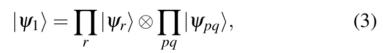
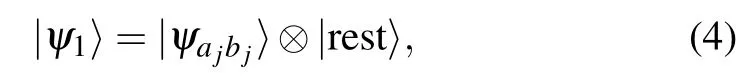
where|ψr〉is the state of qubit r,|ψpq〉is an entangled state of qubits p and q,and the indices r and p,q do not overlap. This conclusion is drawn with the following proven fact. If a projection operator Πjprojects onto an entangled state of qubits ajand bj, then the solution has either of the following two forms:

In the quantum algorithm of Ref. [16], Farhi et al. constructed a Hamiltonian
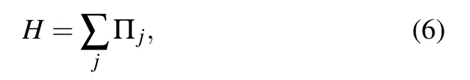
where Πjis of the form in Eq.(2). There is one-to-one correspondence between the solutions of a Q2SAT problem and the ground states of its corresponding Hamiltonian. To see this,we consider a state |ψ2〉. If a state |ψ2〉 is a solution of the Q2SAT problem,then
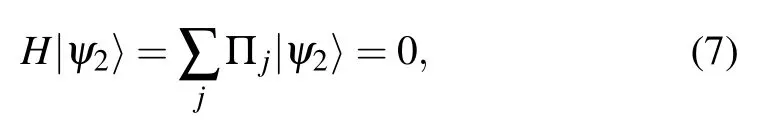
and if|ψ2〉is not a solution,then
Therefore, |ψ2〉 is a solution of the Q2SAT problem if and only if it is a ground state of the Hamiltonian H. The state is initialized to
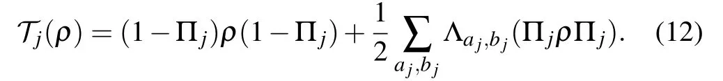
In each step of the algorithm, a projection operator Πjis selected and measured at random. If the result is 0, then do nothing, otherwise a Haar random unitary transfromation is applied,
on one qubit ajof the two qubits ajand bjinvolved in Πj.That is,the operation on the state in each step is
where
Now set
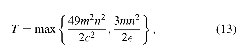
where c(n) is the energy of the ground state and ∊(n) is the energy gap between the ground state and the first excited state.It is assumed that ∊(n) ≈n−g(g positive). After steps of length T, the algorithm has a probability of at least 2/3 to produce a state ρTwhose fidelity with the solution is at least 2/3. The quantum algorithm has a time complexity of at least O(mn2/∊),and gives a non-trivial solution.
4. Our algorithm
Our algortihm follows the one proposed in Ref.[10]. For a Q2SAT problem of n qubits and m two-qubit projection operators{Π1,Π2,...,Πm},we construct a Hamiltonian similar to Eq. (6)
where we have replaced |α| with
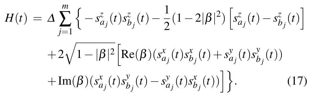
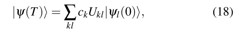
It is obvious that the eigen-energies of H(t)do not change with t and the corresponding eigenstates can be obtained by rotating those of H0. Specifically, the energy gap δ(n) between the ground states and the first excited states does not change with t. We are interested in the adiabatic rotation,where T is big enough. In this case, according to Ref. [17], if the initial state |ψ(0)〉 lies in the subspace spanned by the degenerate ground states{|ψk(0)〉},i.e.,|ψ(0)〉=∑kck|ψk(0)〉,then the final state|ψ(T)〉lies in the subspace spanned by the ground states{|ψk(T)〉}as well. Specifically,we have
where
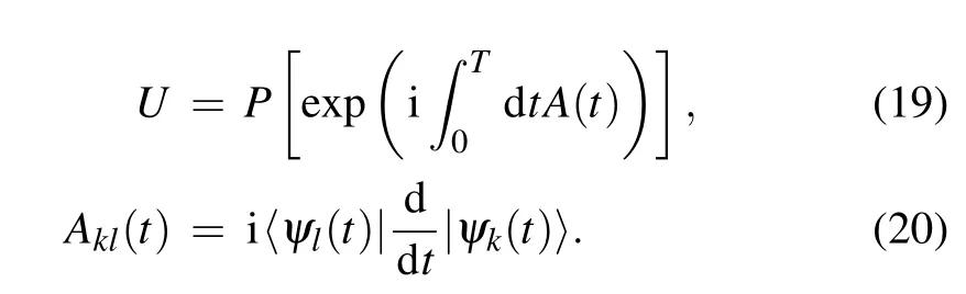
Here A is the non-Abelian gauge matrix that drives the the dynamics in the subspace of the degenerate ground states. For
Here is our algorithm.
• Choose a trivial solution of the Q2SAT problem as the initial state|ψ(0)=|00···00〉and set H(0)=H0.

• Make measurement at the end.
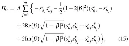
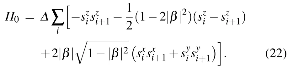
As shown in Ref.[3], the time complexity of a quantum adiabatic algorithm is proportional to the inverse square of the energy gap δ(n) between the ground states and the first excited states. So,the time complexity of our algorithm depends on how the energy gap δ(n)scales with n. Here we consider a special case to estimate the energy gap and examine how it is influenced by the coefficient|β|. In this special case,the spins form a one-dimensional chain and couple to their two neighbors. We assume that β is a positive real number. The special case is in fact the well known Heisenberg chain and has been thoroughly studied. Its Hamiltonian is
5. Numerical simulation
In our numerical simulation,we focus on the special case where
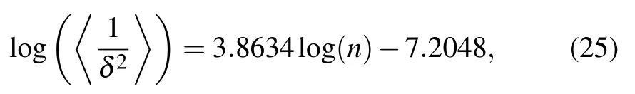
with correlation coefficient r = 0.995. This shows that the inverse square of the energy gap 〈1/δ2〉 ≈O(n3.9) and the time complexity t ≈O(n3.9) according to Ref. [3]. Such a time complexity is better than that of the quantum algorithm in Ref. [16], which is of O(n5.9) for m ≈dn(n −1)/2 and 1/δ ≈O(n1.9).
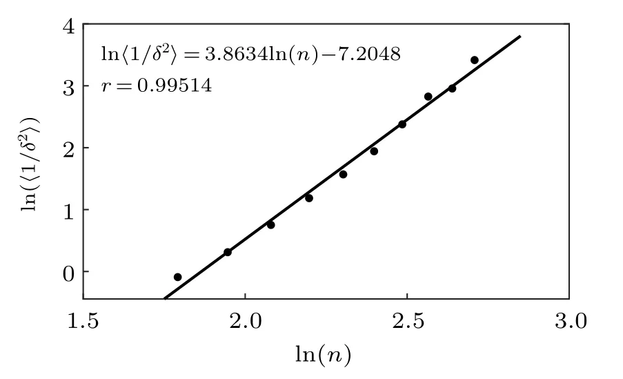
Fig.1. The relation between the average of the inverse square of energy gaps of randomly generated problems and the number of qubits. The x-axis is the logarithm of the number of qubits, log(n), and the y-axis is the logarithm of the average of the inverse square of the energy gap,log(〈1/δ2〉). The line is fitted by least squares method.
Shown in Fig.2 is the distribution of the inverse square of energy gaps 1/δ2for a group of randomly generated graphs with n=11. The distribution shows that few graphs lead to a large inverse square of the gap,but most problems correspond to small inverse square of the gap near the average. Thus it is reasonable that we use the average of the inverse square of the energy gap to compute the time complexity.
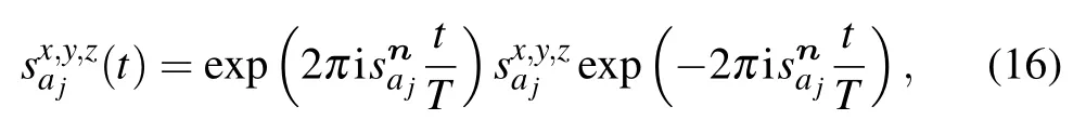
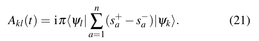
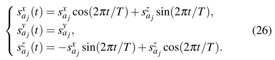
Although our algorithm is quantum,we can still simulate it on our classical computer when the graph size is not very large. In our simulation,we choose the direction ˆn to be along the y-axis. In this simple case,we have explicitly how the spin operators rotate
In our numerics, we choose T = π/(50δ2) for randomlygenerated graphs with n from 8 to 14. We simulate the evolution of the system by the fourth-order Runge–Kutta method,and calculate the module square of the coefficients,i.e.,probability,of the final state on all the possible ground states. The probability of the trivial states for graphs with n from 8 to 14 and the probability distribution for a graph with n=14 are shown in Fig.3. It can be seen that after the adiabatic evolution, we do not return to the trivial state but reach a nontrivial state with a high probability. Such an ability to find a non-trivial solution is better than that of the classical algorithm proposed in Refs.[12,15].
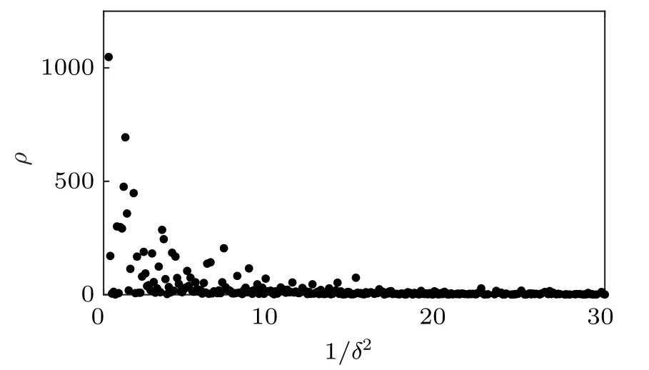
Fig.2. The distribution of the inverse square of energy gaps for 10000 randomly generated problems with n=11. The x-axis is the inverse square of the energy gap,1/δ2,and the y-axis is the number ρ of problems whose energy gap is within[1/δ2 −0.1,1/δ2].
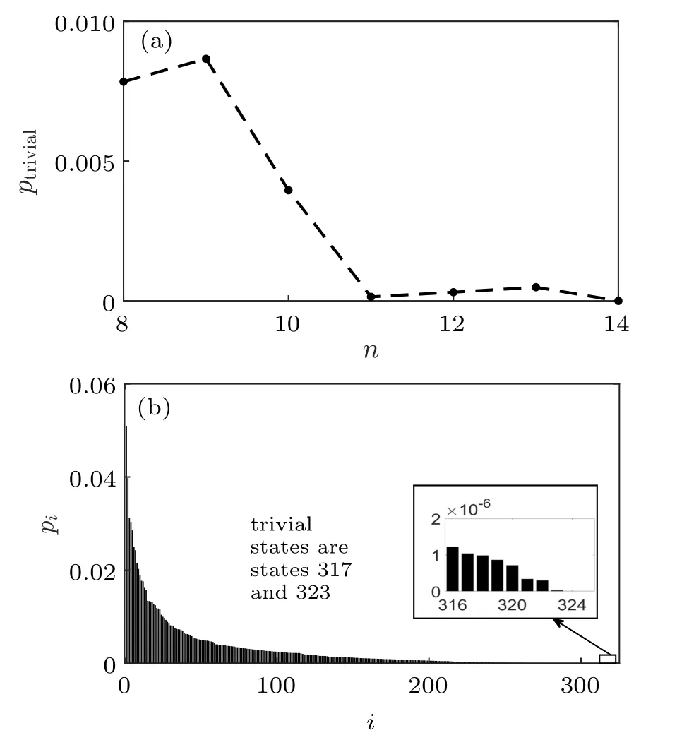
Fig.3. (a) The probability of trivial states of a randomly generated Q2SAT problem after the adiabatic evolution for different n.The dashed line is guide for the eyes. (b)The probability distribution of a randomly generated Q2SAT problem on all its ground states after the adiabatic evolution for n=14. The x-axis is the index of all the ground states.The y-axis is the probabilities of the ground states in the final state.The ground states are indexed according to their probabilities in the descending order. The indexes of the trivial states are 317 and 323.
For our algorithm to work, a large number of solutions are required. However,when d>0.1,the number of solutions decreases significantly. In that case,the state remains on trivial states with a high probability after the adiabatic evolution,and our algorithm thus does not work any more. Numerical results show that for n=14 and d>0.15,our algorithm fails with a non-negligible probability.
6. Conclusion
A quantum adiabatic algorithm for the Q2SAT problem is proposed. In the algorithm,the Hamiltonian is constructed so that all the solutions of a Q2SAT problem are its ground states.A trivial product-state solution is chosen as the initial state.By rotating all the qubits, the system evolves adiabatically in the subspace of solutions and ends up on a non-trivial state. Theoretical analysis and numerical simulation show that,for a set of Q2SAT problems,our algorithm finds a non-trivial solution with time complexity better than the existing algorithms.
Acknowledgement
The authors thank Tianyang Tao and Hongye Yu for useful discussions.
猜你喜欢
当代旅游(2022年16期)2022-12-02
公民与法治(2022年10期)2022-10-12
环球飞行(2021年9期)2021-09-28
广西电业(2020年9期)2021-01-12
少儿美术(快乐历史地理)(2019年3期)2019-07-23
绿色科技(2019年7期)2019-05-23
晚晴(2017年9期)2017-09-21
视野(2016年2期)2016-02-03
天文爱好者(2015年12期)2015-08-23
新西部(2014年10期)2015-01-05

- Chinese Physics B的其它文章
- Novel traveling wave solutions and stability analysis of perturbed Kaup–Newell Schr¨odinger dynamical model and its applications∗
- A local refinement purely meshless scheme for time fractional nonlinear Schr¨odinger equation in irregular geometry region∗
- Coherent-driving-assisted quantum speedup in Markovian channels∗
- Quantifying entanglement in terms of an operational way∗
- Tunable ponderomotive squeezing in an optomechanical system with two coupled resonators∗
- State transfer on two-fold Cayley trees via quantum walks∗