Investigation of bright and dark solitons in α,β-Fermi Pasta Ulam lattice

Nkeh Oma Nfor, Serge Bruno Yamgou´e, and Francois Marie Moukam Kakmeni

1Department of Physics,Higher Teacher Training College Bambili,The University of Bamenda,P.O.Box 39,Bambili-Cameroon

2Complex Systems and Theoretical Biology Group,Laboratory of Research on Advanced Materials and Nonlinear Science(LaRAMaNS),Department of Physics,Faculty of Science,University of Buea,P.O.Box 63 Buea-Cameroon

Keywords: Fermi Pasta Ulam,paradox,bright,dark

1. Introduction

Nature provides many examples of coherent nonlinear structures and wave patterns.Among these beautiful nonlinear phenomena are localized large amplitude solitary waves called solitons, which have been observed in neural networks,[1–3]optical fiber systems,[4–6]and many other physical regimes.Solitons can propagate along one direction over long distances without spreading,and maintaining their form after collision.This particle nature of soliton represents one of the most striking and exciting aspects of nonlinear waves. Solitons are a continuous source of fascination for the physicist, with the Fermi Pasta Ulam(FPU)chain serving as their birth place.[7]

Enrico Fermi initially brought up the idea of investigating on the dynamics of atoms in a crystal,by theoretically considering a long chain of particles linked by Hookian springs.[7]It is important to note that for purely linear springs, the energy given to a single normal mode is only maintained in that mode. Consequently, Fermi further considered weak nonlinearity in the chain by incorporating quadratic nonlinearity in the case of α-FPU model,[8]or cubic nonlinearity for β-FPU model.[9]Due to this nonlinear correction, Fermi, Pasta, and Ulam were confident that the energy introduced into the lowest frequency mode(k=1)would eventually excite other higher modes until the entire system attains a configuration of energy equipartition.[10–12]At the initial phase of the investigation, some higher frequency modes (i.e., k=2, k=3,...)seemed to successfully reached a state close to energy equipartition. However when they accidentally forgot the system to run overnight, it was surprisingly observed the next day that after remaining in the quasi equipartition for a while, almost all the energy of the system returned back to the lowest frequency mode.[13]This experiment was rigorously repeated with faster computers, and the results clearly confirmed the super-recurrence phenomenon in which the initial state was recovered with high degree of precision.[14,15]In fact,this was a ground breaking result and termed the FPU paradox,because the anharmonicity introduced in the lattice could not ensure energy equipartition.

The FPU paradox triggered intense debate in the scientific community with several schools of thoughts to elucidate on this strange phenomenon. The solution of the paradox was tackled in two fronts,i.e.,based on the Kolmogorov–Arnold–Moser (KAM) theory and the soliton concept. The KAM theory became quite reliable in clarifying the recurrence phenomenon of normal modes in the FPU chain, by postulating that most orbits of a slightly perturbed integrable Hamiltonian system exhibit quasi-periodic motion. Even though no qualitative estimate of the recurrence time has been realized based on this theory,recent studies with β-FPU lattice revealed that Birkhoff normal forms compose of an integrable approximation of the FPU Hamiltonian with the integrals physically depicting the linear energies of the normal modes.[16]Izrailev and Chirikov exploited the concept of overlap of nonlinear resonances and further extended the KAM orbit theory by predicting that an increase in the nonlinearity of the FPU chain naturally enhances the rapid equipartition of energy because of the chaotic nature of the orbits.[13,17]The remarkable theoretical arguments put forth by KAM theory and other related theories greatly illuminated some intricacies surrounding the FPU paradox, but were limited with concrete experimental backings. The soliton theory which deals with localization in real space, but also extended in Fourier spaces, naturally became a very powerful tool to explain the paradox as highlighted below.

By using the continuum limit approximation in 1965,Zabusky and Kruskal eloquently explained the recurrence phenomenon by introducing the soliton concept.[18]Their investigation was based on the α-FPU lattice, in which the robust nature of Korteweg–de Vries(KdV)solitons in space coordinate system gave satisfactory answers to the recurrence phenomenon. Upon imposing periodic boundary conditions in the FPU lattice, it was observed that the generated solitons continually move and collide at these boundaries, come back to their initial positions with their shapes unalter (recurrence phenomenon).The explanation of the recurrence phenomenon also gave a sound theoretical answer to the solitary wave discovery by John scott Russel in 1834.[20]The remarkable result obtained by Zabusky and Kruskal has greatly motivated our current investigation, because we seek to extend their studies by adding the cubic nonlinear force term(β-term). In fact,we look for bright and dark solitons of the extended Korteweg–de Vries (eKdV) equation and establish the conditions for their existence. This study seeks to qualitatively extend the argument of the FPU paradox by relating it to the phenomenon of modulational instability in the lattice. The FPU paradox thus forms the foundation for all the powerful theories in solitons and chaos. This explains why the commemoration of the 50th anniversary of Los Alamos FPU report took place in 2005,where scientists around the world organized numerous seminars and conferences to ponder over their research results.[19]

In Section 2, we will establish the equations of motion that emanate from the α,β-FPU chain. This will be followed by deriving the eKdV equation and then the nonlinear Schr¨odinger(NLS)amplitude equation. The modulational instability analysis will be carried out in Section 3 to establish the conditions for observing bright and dark solitons in the lattice. Analysis in Section 4 will be focused on analytically obtaining the bright and dark solitons,followed by investigating on their propagation and collision. In Section 5,we will summarize the important results obtained and articulate on some brighter perspectives.

2. Model equations

Fermi,Pasta,and Ulam considered the simplest model of a discretized nonlinear string, which can also be interpreted as a model of a one-dimensional crystal. It is actually a onedimensional chain of equal particles, fixed at both ends, with each particle experiencing nearest-neighbor interactions.Such interactions are nonlinear in nature. We denote by qjthe displacements of the particles from their equilibrium positions,and pjthe corresponding momenta,for j=1,...,N,with the boundary conditions given by

The Hamiltonian of the system is thus given by

where pj=m ˙qjis the momentum. m is the mass of each identical particle,and V is the potential of interaction of the particles with the nearest-neighbors. The force resulting from the interaction of the springs is given with a certain precision in the following form:

where K, α, β are respectively the linear, quadratic nonlinear,and cubic nonlinear coupling coefficients. Taking into account the fact that the force resulting from the interaction of the springs is derived from the potential (i.e., F =−gradV);we can easily obtain the interaction potential of the system as

The canonical equations of Hamiltonian(2)are given by

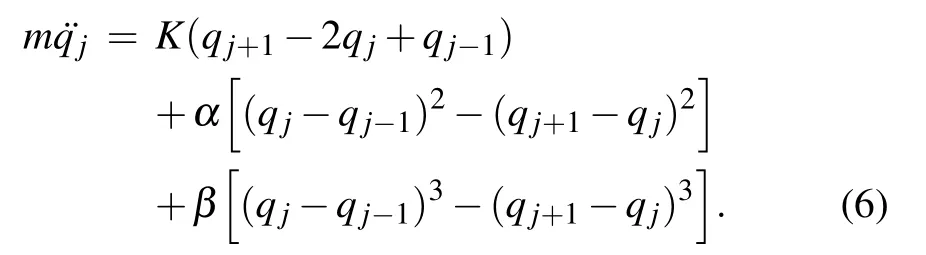
which lead to the discrete equation of motion in the form

2.1. The extended KdV equation

Martin Kruskal and Norman Zabusky considered the Taylor series expansion of qj±1to obtain[18]

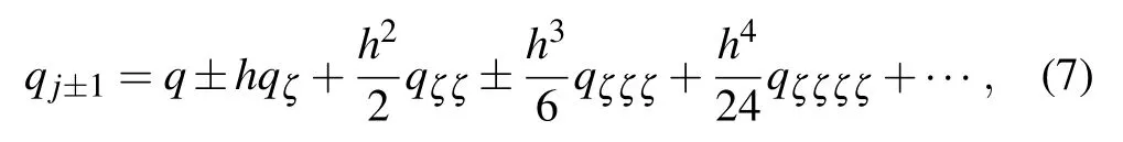
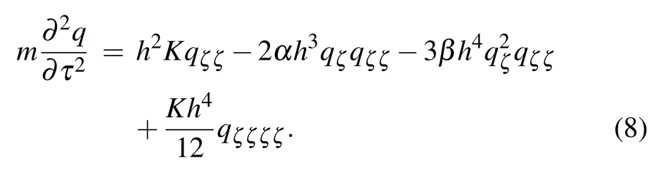
where q=q(ζ,τ)is a displacement of the infinitely small part of the chord with coordinate ζ at time moment τ, and h is a small parameter. Upon substituting expansion (7) into the system of Eq.(6),we derive a partial differential equation for the description of the system dynamics in the continuous limit approximation as

By introducing the new parameter

and imposing the scaling transformations

equation(8)can be re-written as

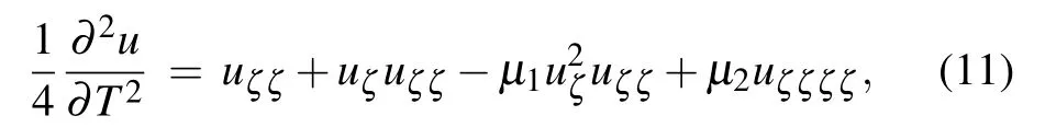
in which function θ(x,t) corresponds to the long distance wave profile. It is important to remark that since ε ≪1, we will generally neglect terms of higher orders in ε. Then using relation(12),equation(11)is transformed to

Without loss of generality,we set ε=1 and use a new variable

in order for Eq.(13)to take the form

Equation (15) is the eKdV equation,[22]where the second and third terms respectively introduce the quadratic and cubic nonlinearities in the system, while the last term with coefficient µ2represents the dispersive term. φ(x,t) is the amplitude of the relevant wave mode, x a horizontal coordinate in a frame of reference moving with the appropriate linear long-wave speed, and t is time. For µ1=0 (i.e., β =0),one naturally obtains the KdV equation that governs the nonlinear dynamics of α-FPU lattice and used by Zabusky and Kruskal to explain the FPU paradox,[18]and also models the dynamics of ion-acoustic wave in plasma.[24–26]The eKdV and µ2=Eq.(15)admits a plethora of solutions. This includes rational solutions,[27–29]rogue wave-type solutions,[31–33]and breather solutions.[23]It should be noted that the KdV and eKdV equations are special cases of a more general variable-coefficient compound Korteweg–de Vries–Burgers equation,used in solid state physics and fluid dynamics.[34–36]

2.2. Derivation of the nonlinear Schro¨dinger amplitude equation

Numerous pulse solutions obtained for Eq. (15) do not properly describe all the excitations in the α,β-FPU chain.We now seek to go further by looking for more appropriate solutions of the eKdV equation that give a comprehensive description of modulated waves in the α,β-FPU chain. Such solutions made up of carrier waves modulated by envelope signals are ubiquitous for most weakly nonlinear systems and described by a wave equation in the small amplitude limit.The method of multiple-scale expansion, in which both the carrier waves and the amplitude are treated in the continuum limit, is a very suitable method used to obtain the amplitude equations.[37–39]

According to the reductive perturbative technique, we consider the ansatz for the solution φ of the form[40]

where the amplitudes A,B,C and their complex conjugates A∗,C∗are functions of X =εx and T =εt. We have θ =κx−ωt,where κ represents the normal wavenumber,ω stands for the angular frequency,and ε ≪1 is a small perturbation parameter.

The ansatz(16)is substituted into the eKdV Eq.(15),and grouping terms in order of perturbation ε0,ε1,ε2,...and various harmonics(i.e., einθ,for n=0,1,2,...)leads to the following results.

Harmonic terms in e0iθat the third-order of approximation ε3yield

Collecting terms of order ε eiθgives

which leads to the group velocity

All the other first harmonic terms that include components in the order of perturbation ε2and ε3lead to

By introducing the frame of reference moving with the group velocity,i.e.,ξ=X −vgT,and imposing τ=εT,equation(20)is then modified;we obtain an equation in the order ε3as

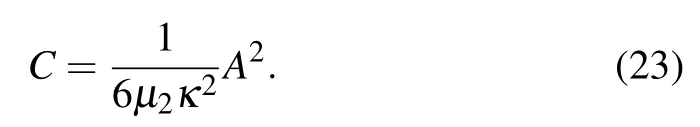
We deduce from the reference coordinate system that ∂/∂T =−vg∂/∂X+···,which is used to simplify Eq.(17)in order to have

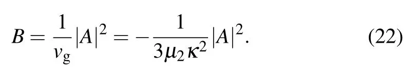
We also collect terms of the order ε2e2iθand simplify to have

Finally, upon substituting relations (22) and (23) into Eq.(21),we obtain the classical nonlinear Schr¨odinger(NLS)amplitude equation given by

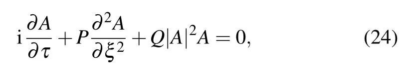
where

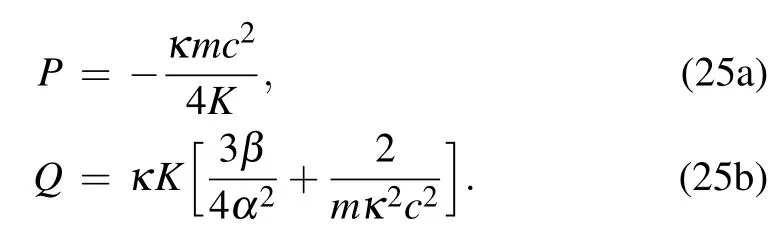
The dispersion coefficient P and nonlinear coefficient Q generally depend on the parameters of the particular system under investigation. In the present case, P and Q depend on wavenumber κ, mass m, and arbitrary constant c. They are also inextricably linked to the constants K,α,β,which are respectively the linear, quadratic nonlinear, and cubic nonlinear coupling coefficients. The NLS equation is a well-known model for the evolution of weakly nonlinear quasi-harmonic wave packets,and prominent in modelling the propagation of electromagnetic waves in optical fibers, among other myriad of applications. The proceeding section will be focused on the modulational instability analysis of the system,which is a very useful technique in determining the conditions for the existence of both bright and dark solitons in the α,β-FPU chain.

3. Modulational instability analysis

Haven derived the NLS amplitude Eq.(24),we now consider the instabilities of continuous waves with respect to small modulations in amplitude or phase, which take place in conservative systems. Since the discovery by Benjamin and Feir in 1967,[41]modulational instabilities(MI)have played a vital role in diverse areas of scientific research. Generally,MI can be considered as a precursor for energy localization in nonlinear lattices like the α, β-FPU chain. MI is responsible for many physically interesting effects such as the break-up of deep water-gravity waves in the ocean,the formation of bright solitons in optical fibers and nonlinear electrical transmission lines,[4,5]as well as the observation of localized nonlinear excitations in neural networks.[1–3]

The plane-wave solution to the NLS Eq.(24)can be written in the general form

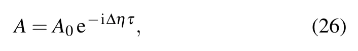
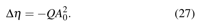
where ∆η is the frequency shift, and A0is the amplitude of the plane wave which is assumed real. The dispersion relation associated with the plane wave(26)is given by

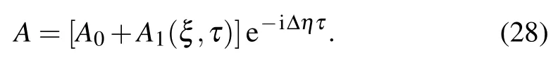
We now monitor the evolution of the plane wave solution in the lattice by considering small perturbations A1(ξ,τ) (i.e.,|A1|≪A0)on the amplitude of the plane wave such that

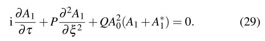
Using Eqs. (24), (27), and (28), we obtain the following linearised equation in A1(ξ,τ):

At this stage, we decompose A1(ξ,τ) by means of the transformation A1=a+ib,in order to respectively obtain the real and imaginary equations as

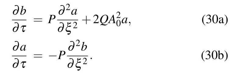
Finally,we now seek solution to Eq.(30)of the form

where k1and Ω are the wavenumber and frequency of the small perturbation, respectively. After some calculations, we now obtain the dispersion relation of the form

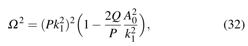
which is now very clear that the stability of the continuous wave depends critically on the sign of Q/P.

Consequently,the wavenumber k1falls in the range

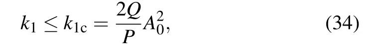
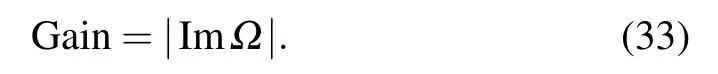
with the maximum growth rate given by

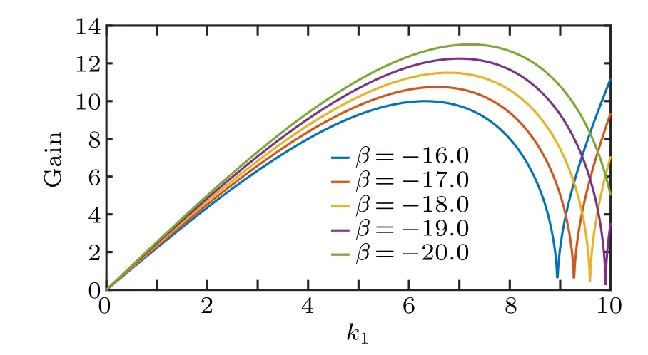
Fig.1. Instability growth rate according to Eq.(33)for different values of β parameter. This is for κ =m=c=α =A0=1.00.

Figure 2 depicts the contour plot for the variation of the β parameter with the wavenumber κ,when the product PQ is computed. To appropriately understand the influence of this β parameter and wavenumber κ on the dynamics of both bright and dark solitons in the α,β-FPU lattice,it is important for us to highlight the following.

For values of β in the range (0 ＜β ≤−20), and low wavenumber κ (i.e., 0 ≤κ ≤1.60), the product PQ is still negative with the predominance of dark solitons in the lattice.However when κ becomes large(1.60 ≤k ≤4.0),PQ becomes increasingly more positive,hence strongly indicating the existence of bright solitons in the α,β-FPU chain.

For β =0 and for any value of the wavenunber κ, the product PQ is always negative indicating stability of the plane wave solutions. Hence information is purely conveyed in the form of dark solitons in the α-FPU chain.

For β >0,the product PQ is always negative irrespective of the values of the wavenumber κ.This strongly suggests that the existence of bright solitons is guaranteed in the α,β-FPU chain only for negative values of β parameter.

Figures 1 and 2 clearly capture and crystallize the MI characteristics in the FPU lattice,hence giving us a clear picture on the evolution of plane wave solutions into solitons.The next section is entirely devoted in tracing the propagation of these solitons in the α, β-FPU lattice, since we have clearly established the appropriate conditions for their existence.

Fig.2. Variation of the product PQ of Eq.(25)for m=c=α =1.00.

4. Propagation and collision of bright and dark solitons in the lattice

In the previous sections, we derived the eKdV and NLS amplitude equations and showed that the observation of bright and dark solitons in the α,β-FPU chain is inextricably linked to the phenomenon of MI.In this section,we will analytically obtain the bright and dark solitons,and numerically investigate on their evolution.

It is very important for us to refresh our minds on the remarkable results obtained by Martin Kruskal and Norman Zabusky,[18]to successfully explain the FPU paradox. Since they were working with the α-FPU lattice, they obtained the KdV equation written in the form

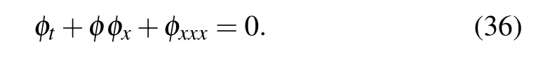
The KdV Eq.(36)is very important in nonlinear science,not only because of its pioneer role but also because it is able to describe many physical phenomena including blood-pressure pulse propagation. A careful observation shows that the KdV Eq.(36)is derived from the eKdV Eq.(15)by setting µ1=0 andµ2=1,without loss of generality.Equation(36)is a blend of nonlinear hyperbolic term φφxand a linear dispersive term φxxx. Among other solutions admitted by the KdV Eq.(36)are travelling waves solution of the form[37]

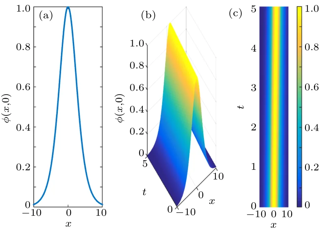
Fig.3. Propagation of KdV pulse solution(37)for φ0=1/.

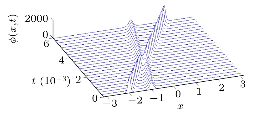
Fig.4. The three-dimensional KdV pulse soliton collision.

The bright and dark solitary waves provide favorable alternatives for transmission of signals in nonlinear systems,like discrete electrical and mechanical lattices.[42–45]For example,the form of matter-wave solutions of Bose–Einstein condensates with three-body interaction depicts a dark-like profile.[46]However in dissipative systems like lossy optical fibers,bright solitary waves are more susceptible to fiber losses because of the high decrease of wave amplitude and increase in width during propagation down the waveguide. Such losses are highly minimized with the transmission of dark solitary waves down the optical fiber.[47]By using the ansatz (16), we successful showed in Section 2 that the eKdV Eq.(15)admits both bright and dark solitons under specific conditions. We now seek to further explain the recurrence phenomenon for the α,β-FPU lattice by investigating on the evolution of these bright and dark solitons that emanate from the NLS amplitude Eq.(24).

4.1. Bright soliton

For PQ>0, the envelope-soliton solution of Eq. (24) is given by[38,48]

where the amplitude ψ0and the width Leof the bright soliton are given by

It is useful to stress that u2e−2ueup>0,where ueand upare the velocities of the envelope and carrier waves, respectively,while the amplitude ψ0varies with the β parameter as shown in Fig.5.As β decreases from −2.0 to −20.0,we observe that the amplitude gradually decreases and the pulse slows down and becomes broader. Figure 6 depicts the evolution of the magnitude of the bright soliton solution(38)for a fixed value of β, it manifests the same structural features as with their KdV counterparts shown in Fig.3. The profile of the bright solitons in Fig.6 also resembles the first-order bright solitary waves observed in the non-autonomous generalized AB system.[31]

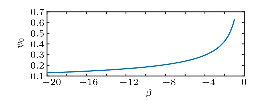
Fig.5.Variation of bright soliton amplitude(39)with β parameter.This is for m=c=α =ue=1.00,up=0.25,and wavenumber κ =4.0.

Fig.6. Propagation of the magnitude of bright soliton solution (38).This is for P=Q=ue=1.00,up=0.25,ψ0=0.50,and Le=2.83.

By using the pseudo-spectral numerical scheme with P=1.0, Q=2.0, and step sizes dτ =0.02, dξ =0.31, we now numerically integrate Eq.(24)with initial conditions given by considering solution(38)at τ=0.0;this leads to exciting collision phenomena manifested in Figs. 7 and 8. In Fig.7, a bright soliton moving to the right collides with another stationary bright soliton at the origin.The two solitons cross each other just with a slight phase shift, consequently their shapes and amplitudes are conserved after the collision process. This result is consistent with the observation made by Zabusky and Kruskal as shown in Fig.4. On the other hand, we also consider two solitons moving in opposite directions as shown in Fig.8. Upon colliding at their boundaries,they are redirected and eventually lead to collisions around the origin. The robust wave packets still maintain their amplitude and shape after these multiple collisions,hence consistent with the recurrence phenomena and reinforcing John scott Russel observations.[20]

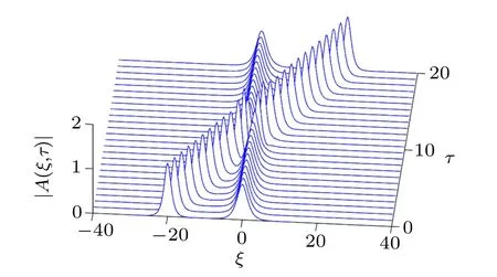
Fig.7. Single collision of bright solitons given by solution (38) for P=1.0,Q=2.0.

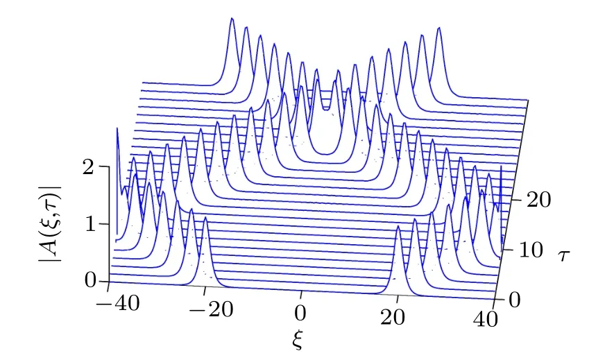
Fig.8. Multiple collisions of bright solitons,with the same parameters as those in Fig.6.

Let us now consider the appropriate bright soliton solution of the eKdV Eq. (15) by substituting solution (38) into the ansatz(16),in order to obtain

where

Figures 9 and 10 show the evolution of bright solitons in the FPU lattice at different time, for some fixed values of the system parameters. In Fig.9, we clearly see that the wave envelope propagates to the right and maintains its amplitude of approximately 1.0, with the shape of the wave envelope unchanged. This clearly depicts the classical behavior of a soliton as initially observed by John scott Russel.[20]However when the perturbation parameter ε is set to 0.10 as in Fig.10,the wave becomes broader and still maintains its shape during propagation. This strongly suggests that variation in the external perturbations is inextricably linked to changes in the speed of bright solitons.

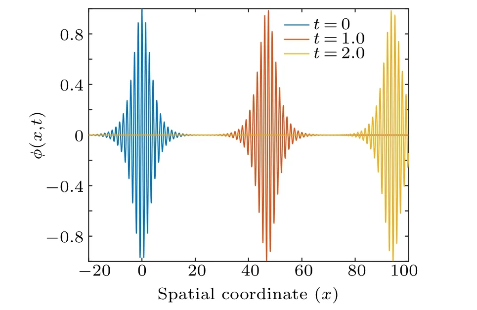
Fig.9. Propagation of bright soliton of the eKdV Eq.(15). This is for P=Q=ue=1.00,up=0.25,ψ0=0.50,Le=2.83,µ2=1.0,κ=4.0,and ε =1.0.

Fig.10. Propagation of bright soliton of the eKdV Eq. (15), with the same parameters as those in Fig.9 but for ε =0.10.

4.2. Dark soliton

It is now incumbent on us to complete the findings by demonstrating the existence of dark solitons in the FPU lattice. As a reminder, dark soliton was discovered in 1973 by Hasegawa and Tappert.[49]It has already been analytically and experimental demonstrated in many physical regimes ranging from optical fibers,[49,50]plasmas,[51]to aquatic environment.[52]Such a wave profile is equally ubiquitous in discrete lattices, and appears as dips in the stable constant-wave background.[53,54]

For PQ ＜0,an envelope soliton can not propagate in the α, β-FPU lattice, but a dark soliton does. According to the analysis in Ref. [38], the dark soliton solution of Eq. (24) is given by

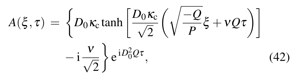
where ν is the common velocity for both the carrier and envelope,D0and κcare arbitrary constants. Figure 11 depicts the propagation of the magnitude of dark soliton solution(42) to the left,characterized by a constant dip.[31]As highlighted in Ref. [38], κcdetermines the value of ν and for κc=1.0, the velocity ν vanishes. Hence solution(42)degenerates to

with the dark soliton solution of the eKdV Eq.(15)given by

where

Fig.11. Propagation of the magnitude of dark s√oliton solution (42√) to the left.This is for P=−1.0,Q=1.0,D0=ν=,and κc=1/.

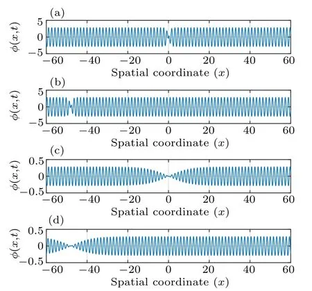
Fig.12. Propagation of dark soliton solution (44), in the FPU lattice.This is for P=−1.0,Q=1.0,D0=√,κ =4.0,and µ2=1.0. (a)ε=1.0,t=0.0;(b)ε=1.0,t=1.0;(c)ε=0.10,t=0.0;(d)ε=0.10,t=1.0.

Figure 12 shows a finite amplitude continuous wave which is partially modulated by sinusoidal waves of low frequency, propagating to the left of the lattice. Concretely, figure 12(a)gives the initial profile of the wave(i.e.,ε =1.0,t=0.0), where the amplitude or envelope function of the soliton has a hole at the origin x=0. On the other hand,figure 12(b)shows the stable propagation of the dark soliton toward the left of the FPU chain to a new position, i.e., the center of the dark soliton is now moved to a new position at x=−50 after time t =1.0. When the perturbation parameter ε is slightly changed to 0.10 as in Figs.12(c)and 12(d), the dark solitons exactly move as in Figs. 12(a) and 12(b), but with the amplitude and shape of the wave slightly modified. In fact, we observe a more modulated wave profile with a shallow depth.

5. Conclusion

We investigated on the dynamics of bright and dark solitons in the α,β-FPU chain,in order to elucidate on the FPUparadox. The Hamiltonian formalism was used to obtain the relevant equation of motion,from where we derived the eKdV equation used in the description of wave processes in the lattice. In fact, the robust soliton solutions of the KdV equation were used by Zabusky and Kruskal to resolve the FPUparadox and have triggered enormous research activities in the field of nonlinear physics. We also investigated on the long time dynamics of modulated waves in the α,β-FPU chain via the NLS amplitude equation. In the standard NLS equation,the phenomenon of MI corresponds to the condition PQ>0,where the perturbations of low-amplitude carrier waves provide an instability which ultimately leads to the breaking up of the waves into envelope solitons. These predictions were confirmed by numerical simulations, in which we demonstrated the propagation, collision, and penetration of robust soliton entities in the lattice. An in-depth investigation on the lattice dynamics revealed that, the bright pulses manifested several intrinsic nearly elastic collision phenomena,with transmission events that only led to a slight phase shift. That is,the pulses emerge out of the collisions without any significant change in their direction of motion, velocities, and shapes. The major exceptions were at the boundaries of the physical domain where we imposed periodic boundary conditions, that led to the reflection of the bright solitons back into the medium with velocities opposite to the ones they had prior to the collision.Furthermore, contrary to the NLS-type MI, the stability observed for PQ ＜0 leads to the generation of hole solitons(dark solitons) in the lattice. We have successfully resolved the FPU-paradox using the MI phenomena and shown that the sign of the nonlinear cubic parameter, β,plays a very crucial role.

In perspective, the study of nonlinear lattice dynamics like the FPU problem is also very applicable in the fields of statistical and solid state physics.For example,in trying to understand the onset of melting in a solid as the temperature of the solid increases, the amplitude of oscillations of the atoms or ions about their equilibrium positions increases and anharmonic contributions become increasingly more important. At some critical temperature,the oscillations are so large that the solid transforms into a liquid.A good mastery of nonlinear lattice dynamics is thus inevitable, in order to comprehensively explain all the physical changes taking place.

Acknowledgement

Our interactions with some students of the department Physics, HTTC Bambili of the University of Bamenda, are greatly appreciated.