
Propagation properties and radiation force of circular Airy Gaussian vortex beams in strongly nonlocal nonlinear medium∗
2021-03-11 08:32XinyuLiu刘欣宇ChaoSun孙超andDongmeiDeng邓冬梅
Chinese Physics B 2021年2期
Xinyu Liu(刘欣宇), Chao Sun(孙超), and Dongmei Deng(邓冬梅)
Guangdong Provincial Key Laboratory of Nanophotonic Functional Materials and Devices,South China Normal University,Guangzhou 510631,China
Keywords: optical vortices,abruptly autofocusing,radiation force,strongly nonlocal nonlinear
1. Introduction
Abruptly autofocusing (AAF) beams have been studied both theoretically[1]and experimentally.[2,3]The focusing mechanism of AAF beams is entirely different from that of Gaussian beams. In the case of Gaussian beams, the wave’s constituent rays form a sharpened pencil which converge at the focus point and as the beam’s cross-sectional area gradually decreases, the maximum intensity over the transverse plane increases in a Lorentzian fashion,centered at the focus.[4]But in the case of AAF beams, the rays responsible for focusing are emitted from the exterior of a dark disk on the input plane and stay tangent to a convex caustic surface of revolution that contracts toward the beam axis.[1]The AAF beams maximum intensity remains almost constant during propagation,while close to a particular focal point,they suddenly autofocus, as a result, their peak intensity can increase by orders of magnitude.[1]This AAF property of the AAF beams is quite useful, which can be used to trapping or guiding microparticles[3,5]and generation of light bullet.[6]
In 1989, Coullet found the vortex solutions of the Maxwell–Bloch equations and created the concept of optical vortices (OVs), inspired by hydrodynamic vortices.[7]Abruptly autofocusing vortex beams were investigated by Jeffrey A. Davis, who gave explicit equations for the phaseonly Fourier masks that generate these beams including explanations for controlling the focal distance and numerical aperture.[8]In recent years, OVs have potential application in the fields of optical communications,[9]high resolution imaging,[10]and optical tweezers.[11,12]
What is more, the propagating properties of all kinds of beams and light bullets in strongly nonlocal nonlinear medium(SNNM) have been exploited, such as Laguerre–Gaussian beams,[13]Airy beam,[14]airy light bullets,[15]and Airy–Laguerre–Gaussian light bullets.[16]In addition to this, a lot of researchers have studied the evolution characteristics of the beams in different categories of potentials,including quadratic nonlinear medium,[17]linear index potentials,[18]parabolic potential,[19]highly nonlocal medium,[20]and higher-order power-law potentials.[21]Nevertheless,as far as we know,the AAF properties and the radiation force of the circular Airy Gaussian vortex(CAiGV)beams in SNNM have not been researched. In this paper, the propagating properties and radiation force of the CAiGV beams are researched through numerical simulations.The magnitude of the topological charges and the position of the vortex can change the light spot pattern and the peak intensity contrast. The positions of the autofocusing and autodefocusing planes,the peak intensity contrast,and the radiation force can be tuned by altering the parameter of the incident beam.
The rest of this article is structured as follows. First and foremost in Section 2,we introduce a kind of theoretical model for the CAiGV beams in SNNM. After that in Section 3, the propagation properties of the beams are discussed. Then in Section 4,the radiation force of the beams is studied. Finally in Section 5,the important conclusions are summarized.
2. The theoretical model
The dynamics of the spatial beams propagating along the z-axis in SNNM can be governed by the (2+1) dimensional
with the 2D nonlinear perturbation of the refractive index ∆n being given by
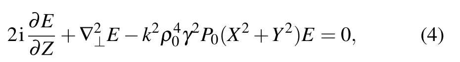
where X and Y represent the normalized transverse coordinates. According to the radially symmetrical CAiGV beams solution,we can describe it in polar coordinates,equation(4)can be rewritten as


The electric fields of the initial CAiGV beams can be expressed as

where A0is the constant amplitude of the electric field; Ai(·)denotes the Airy function;a(0 <a <1)is the truncation factor of the Airy function; R0represents the radius of the first ring of the CAiGV beams;bs(0 <bs<1)is the spatial distribution factor that makes the CAiGV beams tend to the CAiV beams when the spatial distribution factor is small or the Gaussian vortex(GV)beams when the spatial distribution factor is large;(Rk,φk)represents the position of the OVs;(m,l)is the topological charges of the OVs. We cannot obtain the analytical solution for Eq. (5). Fortunately, we can obtain numerical simulations through using the fast Fourier transform method.[27,28]In the following simulation, the related parameters are chosen as A0=1, a=0.1, bs=0.1, m=0, l =0,R0=1,ρ0=100µm,λ =533 nm.
3. Propagation properties of circular Airy Gaussian vortex beams
The side-view intensity profiles of the CAiGV beams are illustrated in Fig.1(a). It is clear that it represents a kind of periodic abruptly autofocusing and autodefocusing evolution behavior.From Figs.1(b1)–1(b5),the transverse intensity profiles are displayed at the planes marked by the dashed lines in Fig.1(a). It can be seen from Fig.1(b1) that the intensity of the annular plate decreases gradually from the inside out and the width of the annular plate also decreases gradually. As the propagation distance increases, almost all the energy focuses on a very small circular light spot region at the autofocusing plane in Fig.1(b2). Comparing Figs.1(b2)and 1(b4),the transverse intensity distribution is the same in the autofocusing plane and the autodefocusing plane. A cylindrical pattern of the light spots is formed between the autofocusing position and the autodefocusing position,and the intensity decreases first and then increases with the increase of the propagation distance,which is due to some interference rings being formed in Fig.1(b3). The transverse intensity distribution in Fig.1(b5)is the same as that in Fig.1(b1),one cycle evolution ending and a new one beginning.
In Fig.2, we analyze the evolution characteristics of the CAiGV beams,one can see clearly a hollow channel,it is because the on-axis vortex(the vortex core of an OV can exist on the propagation axis of the beam,that is to say,Rk=0,φk=0)exists along the propagation. For studying the evolution behavior of the CAiGV beams,we demonstrate the intensity pattern of the CAiGV beams in Fig.2(c).In Fig.2(c),we find that the CAiGV beams can sharply concentrate nearly all energy at the autofocusing plane in SNNM.In Fig.2(d),we describe the phase distribution of the CAiGV beams when the beams exist the on-axis vortex.
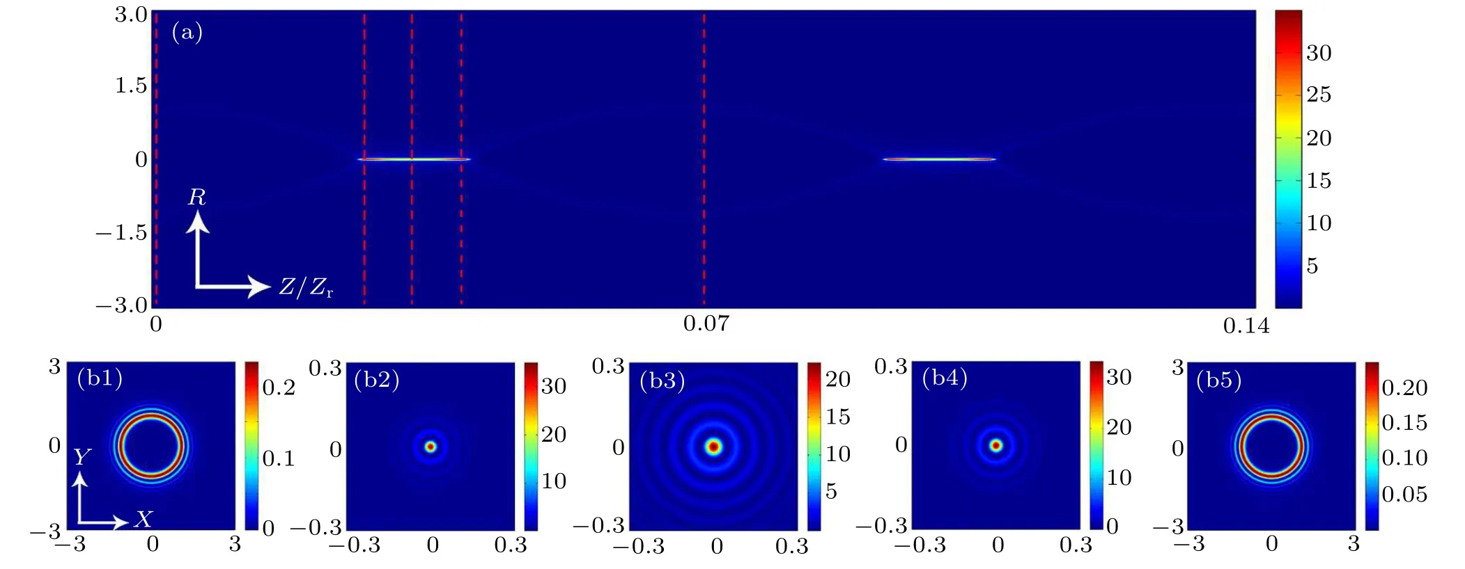
Fig.1. The intensity profiles of CAiGV beams at different propagation distances. (a) The numerically simulated side-view propagation of the CAiGV beams,(b1)–(b5)snapshots of the transverse intensity patterns are taken at the planes marked by the dashed lines in(a).
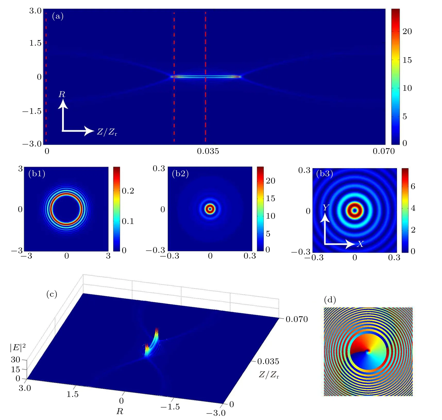
Fig.2. The intensity profiles of CAiGV beams at different propagation distances. (a)The numerically simulated side-view propagation of the CAiGV beams, (b1)–(b3) snapshots of the transverse intensity patterns are taken at the planes marked by the dashed lines in (a), (c) the detailed intensity distribution of the propagation dynamics,(d)the phase pattern at the initial plane. Other parameters are the same as those in Fig.1,except m=1.
In order to study the effect of the spatial distribution factor bsbetter, we plot the transverse intensity profiles and the corresponding cross lines of the CAiGV beams in Fig.3. We can see from Figs. 3(a1)–3(d1) that the CAiGV beams tend to circular Airy vortex (CAiV) beams when bs=0.1, while the CAiGV beams tend to the GV beams when bs=0.5. In Figs.3(a2)–3(d2),the distance between the autofocusing position and the autodefocusing position decreases gradually with the increase of bs, meanwhile, the intensity of the autodefocusing plane increases significantly, as shown in Figs.3(a3)–3(d3).
The off-axis vortices (the vortex core of an OV can not exist on the propagation axis of the beam, that is to say,Rk/=0,φk/=0) are imposed in Fig.4(c). In Fig.4(b1), we can witness a hollow region in which the light intensity is zero on the left of the light spot due to the off-axis vortex,almost all the energy concentrates on the right side of the main ring at the initial plane. As the propagation distance increases,the vortex moves to the center in Fig.4(b2)and all the energy is focused on the center. The intensity profiles rotate 90◦counterclockwise and we can see many interference rings in Fig.4(b3).Compared with the initial plane, the intensity profiles rotate 180◦counterclockwise,as is depicted in Fig.4(b5).
The propagation properties of the CAiGV beams can be noticeably influenced due to the difference of the magnitude of topological charges and the position of the vortex. When we impose two off-axis vortices at the different positions in Figs. 5(a4)–5(b4), the intensity profile of the light spot is the same, but the light spot location is different at the same position. In Figs. 5(a1)–5(b1), the intensity pattern of the CAiGV beam is the shape of a meniscus light spot, and the intensity pattern is a pea-shaped light spot at the autofocusing plane in Figs.5(a2)–5(b2)and at the autodefocusing plane in Figs. 5(a3)–5(b3). When the number of topological charges increases, the light intensity increases, compared to that in Figs. 4(b2)–4(b4). We can find that the intensity contrast increases with the increase of m when we impose on-axis vortices in Fig.5(c), while the intensity contrast decreases first and then increases when we impose the off-axis vortices in Fig.5(d), but the positions of the self-focusing plane and the self-defocusing plane can not change.
Fig.3. The transverse intensity profiles and the corresponding cross lines of the CAiGV beams(a1)–(d1)at the initial plane(Z=0),(a3)–(d3)at the autofocusing plane. (a2)–(d2)The numerically simulated side-view propagation and the corresponding cross lines of the CAiGV beams.Other parameters are the same as those in Fig.2,except bs=0.1 in(a1)–(a3);bs=0.2 in(b1)–(b3);bs=0.5 in(c1)–(c3).
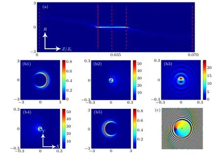
Fig.4. The intensity profiles of CAiGV beams at different propagation distances. (a)The numerically simulated side-view propagation of the CAiGV beams,(b1)–(b5)snapshots of the transverse intensity patterns are taken at the planes marked by the dashed lines in(a),(c)the phase pattern at the initial plane. Other parameters are the same as those in Fig.2,except m=1 and rk=0.8.
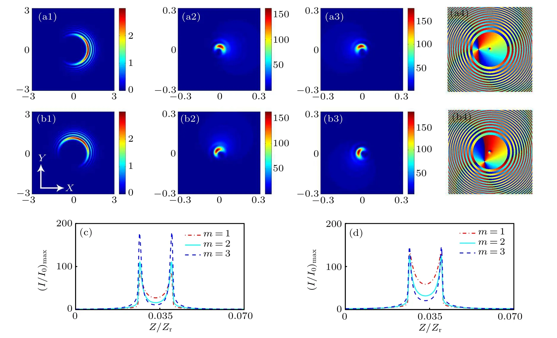
Fig.5. The transverse intensity profiles of the CAiGV beams(a1)–(b1)at the initial plane(Z=0),(a2)–(b2)at the autofocusing plane,(a3)–(b3)at the autodefocusing plane,(a4)–(b4)the phase pattern at the initial plane.Comparison of(I/I0)max of the CAiGV beams with different m as a function of Z for(c)on-axis vortices and(d)off-axis vortices. Other parameters are the same as those in Fig.4,except m=2 in(a1)–(a4),and m=2,φk=π/3 in(b1)–(b4).
Finally, for understanding the effect of the parameter R0and the parameter a better, we depict the peak intensity contrast of the CAiGV beams.One can easily see that the intensity contrast is about the same,but the positions of the autofocusing and autodefocusing in Fig.6(a)can be changed sightly by adjusting the parameter R0, and the distance between autofocusing and autodefocusing decreases with R0increasing. As a increases, the peak intensity contrast of the CAiGV beams decreases in Fig.6(b).
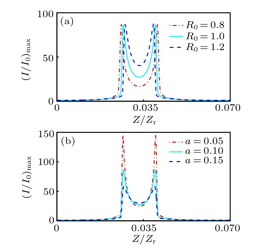
Fig.6. The peak intensity contrast of the CAiGV beams versus the propagation distance for(a)different R0,(b)different a. Other parameters are the same as those in Fig.2.
4. The radiation forces of circular Airy Gaussian vortex beams on a Rayleigh dielectric sphere
Here, we investigate the radiation forces of CAiGV beams on a Rayleigh dielectric sphere in SNNM, which are associated with momentum changes of the electromagnetic wave,and the radius of the Rayleigh dielectric sphere is much smaller than the wavelength of the CAiGV beams (i.e., r0≪λ). When r0≪λ,the Rayleigh dielectric particle can be considered as a point dipole, and the Rayleigh scattering model is used to calculate the radiation forces on the particle.[7]We assume that a micro particle with refractive index npis struck by the CAiGV beams. When the particle experiences a steady state,the gradient force and the scattering force can be calculated by[20]
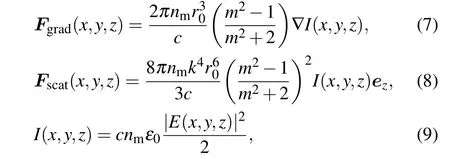
where m=np/nmis the relative refractive index of the particle,nmis the refractive index of an ambient medium,r0is the radius of the micro particle,c is the light velocity,and ε0is the permittivity of vacuum.[30]
In the following text,we choose np=1.592,r0=50 nm.The gradient force and the scattering force are deemed to be two kinds of main radiation forces.[30]From Eq.(7),one can see that the gradient force is proportional to the intensity gradient. From Eq.(8),one can find that the scattering force along the propagation direction is proportional to the intensity.[30]The trapping force can be defined as the sum of the gradient force and the scattering force.There are several necessary conditions for stably trapping in optical traps by CAiGV beams.First, the backward longitudinal gradient force must be large enough to overcome the forward scattering force. Second,the longitudinal gradient force must be large enough to overcome the influences of the buoyancy and the gravity. The third condition is that the potential well of the gradient force must be larger than the kinetic energy of the Brownian particle.[31]It is judged by the Boltzmann factor as follows:[29,32]
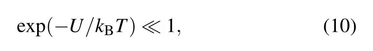
where
is the potential energy of the gradient force at the trap position,kBis the Boltzmann constant,and T is the temperature of the medium,∆I(x,y,z)denotes the intensity difference related with the potential well of the gradient force.[31]
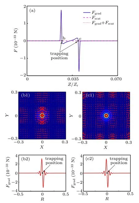
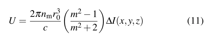
Fig.7.(a)The longitudinal radiation force F on a Rayleith particle with radius of 40 nm versus z;(b1)–(c1)the transverse gradient force pattern(background)and the transverse gradient force flows(red arrows)of the CAiGV beams in the trapping plane; (b2)–(c2)the transverse gradient force in the trapping plane.

Fig.8. The distribution of the radiation force on the Rayleigh particle. (a)The longitudinal gradient force;(b)the scattering force,(c)the sum of the gradient force and the scattering force;(d)–(e)the transverse gradient force in the trapping plane.
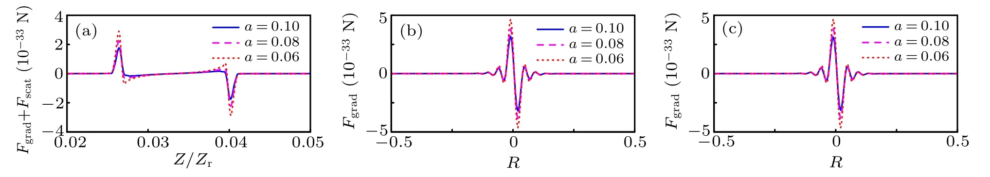
Fig.9. The distribution of the radiation force on the Rayleigh particle: (a)the sum of the gradient force and the scattering force; (b)–(c)the transverse gradient force in the trapping plane.
In order to further investigate the trapping progress, we plot the longitudinal radiation force and the pattern of the transverse gradient force and the transverse gradient force in the trapping plane, as elucidated in Fig.7. In Fig.7(a), one can see clearly that there are two stable equilibrium points in the distribution of the longitudinal trapping force where the Rayleith particle can be trapped. In Figs.7(b1)and 7(c1),one can find that the gradient force vectors in the X-axis is mostly distributed to the left and right,and that in the Y-axis is mostly distributed in the unwards or downwards. From the overall point of view, the gradient force probably presents a circular distribution.Figures 7(b2)and 7(c2)show that the particle can be transversely trapped at b and c.
The distributions of the transverse and longitudinal radiation forces of the CAiGV beams on a Rayleigh particle are elucidated in Fig.8. The scattering force and longitudinal gradient force increase as r0increases and the effective longitudinal trapping force of the CAiGV beams becomes larger. We can also see that the trapping position is slightly shifted forward due to the influence of the scattering force. With the increase of r0, the transverse gradient force also increases in the trapping plane.
Finally, we analysis the distributions of the longitudinal and transverse radiation forces of the CAiGV beams in Fig.9.One can see that the radiation force can be modulated by controlling the parameter a. The longitudinal radiation force and transverse gradient force increase as a decreases,and the trapping position is not changed.
5. Conclusion
We have studied the evolution behavior of the abruptly autofocusing and autodefocusing CAiGV beams in SNNM through numerical calculations. We can see a kind of periodic abruptly autofocusing and autodefocusing evolution behavior, and almost all energy focuses on a very small circular light spot area at the autofocusing plane. The intensity profiles could have a hollow channel when the on-axis vortices are imposed. Furthermore,the CAiGV beams tend to the CAiV beams when bs=0.1 and tend to the GV beams when bs=0.5. Meanwhile,we can change the light spot pattern and the intensity contrast by adjusting the magnitude of the topological charges and the position of the vortex. The intensity contrast increases with the increase of m when the CAiGV beams have on-axis vortices, the intensity contrast decreases first and then increases when the CAiGV beams have off-axis vortices. The intensity pattern of the beams rotates with the increase of the propagation distance, and we can control the position of the autofocusing and autodefocusing planes by adjusting the parameters bsand R0,and we can also change the peak intensity contrast through choosing appropriate a. Finally,we have theoretically investigated the radiation force of the CAiGV beams.One can find that there are two stable equilibrium points in the distribution of the longitudinal trapping force,and we can enhance the radiation force through adjusting parameters of r0and a.

- Chinese Physics B的其它文章
- Novel traveling wave solutions and stability analysis of perturbed Kaup–Newell Schr¨odinger dynamical model and its applications∗
- A local refinement purely meshless scheme for time fractional nonlinear Schr¨odinger equation in irregular geometry region∗
- Coherent-driving-assisted quantum speedup in Markovian channels∗
- Quantifying entanglement in terms of an operational way∗
- Tunable ponderomotive squeezing in an optomechanical system with two coupled resonators∗
- State transfer on two-fold Cayley trees via quantum walks∗