
Constructing reduced model for complex physical systems via interpolation and neural networks∗
2021-03-19 03:21XuefangLai赖学方XiaolongWang王晓龙andYufengNie聂玉峰
Chinese Physics B 2021年3期
Xuefang Lai(赖学方), Xiaolong Wang(王晓龙), and Yufeng Nie(聂玉峰)
Research Center for Computational Science,School of Mathematics and Statistics,Northwestern Polytechnical University,Xi’an 710129,China
Keywords: model reduction, discrete empirical interpolation method, dynamic mode decomposition, neural networks
1. Introduction
Many physical systems and processes in scientific and engineering fields are modeled mathematically by higher-order differential equations.[1,2]Usually, it is time-consuming or even computationally intractable to directly perform simulations on these models. The computational challenge has motivated the development of model reduction. Model reduction is a powerful technique that seeks to approximate the higherorder complex system with a low-order one,aiming at reducing the computational cost with a controlled loss of accuracy.
In this article, we concentrate on the nonlinear systems which are encountered in a wide range of physical phenomena.[3]For nonlinear systems, the existing approaches for model reduction cover quadratic expansion,[4]trajectory piecewise-linear (TPWL),[5,6]piecewise-polynomial representations,[7]proper orthogonal decomposition (POD),[8,9]and so on.[10]Among them, POD is the most popular method. Up to date,a variety of reducedorder models (ROMs) based on the POD method have been developed, including the intrusive ROMs and non-intrusive ROMs. Usually, the non-intrusive ROMs predict the projection coefficients of the POD basis by applying interpolation or machine learning methods, such as neural networks,[11]and Gaussian process regression.[12]In contrast, the intrusive ROMs are constructed by implementing the Galerkin projection,[13]and often are more effective to use the physical knowledge of the governing equations. Unfortunately,the POD-Galerkin method often suffers from instability and nonlinear inefficiency problems.
An efficient method for obviating this problem is sparse sampling. The pioneer works include gappy POD,[14]empirical interpolation method (EIM),[15]best points (missing points)estimation(MPE),[16]discrete empirical interpolation method (DEIM),[17]and so on. The gappy POD was firstly introduced in Ref.[14]for dealing with the“gappy”or incomplete data vector and later extended to the reconstruction of unsteady flow problems in Ref. [18]. EIM[15]and MPE[16]are another two methods developed for efficiently managing the computation of the nonlinearity. MPE is involved with a least-squares minimization problem, and its computational complexity is much higher than that of the EIM architecture to some extent. Especially,the DEIM,[17]as a discrete variant of EIM, shows superior performance in approximating the nonlinearity by using a small,discrete sampling of spatial points.
Although the interpolation points selected by the DEIM method provide a good approximation for the nonlinear function, some information is inevitably lost. To fill this gap, we propose an improved DEIM method by using the technique of linear truncation, denoted by LT-DEIM.More specifically,instead of applying the classical DEIM approach to the nonlinear function directly,our approach computes a linear approximation for the nonlinear function and evaluates the residual via the DEIM. Here, the purpose of the linear approximation term is to extract some information of the nonlinear function.By integrating the linear truncation method into the DEIM,a more accurate approximation of the nonlinear function can be achieved.
The linear approximation term plays a crucial role in the LT-DEIM model, and we construct it by using Taylor’s expansion and dynamic mode decomposition(DMD),[19]respectively. Taylor’s expansion is a powerful technique for the nonlinear model reduction.[4-6]For example, a reduced model of the Navier-Stokes equations was generated in Ref. [20]by combining the quadratic expansion with the DEIM. However, Taylor’s expansion has some limitations when the nonlinear term is unknown or non-differentiable. Moreover, the nonlinear term is a high-dimensional nonlinear vector function, making it hard to compute the Jacobian matrix and select proper expansion points. Thus, the DMD method is also employed to construct the linear approximation term in this work.DMD is an equation-free and data-driven modal decomposition method that has successfully been used for nonlinear model reduction.[21,22]Moreover,DMD shows the marked improvement in the computational speed for evaluating the nonlinearity.
After the ROM has been constructed,we expect to know how accurate this ROM performs. Some assumptions and approximations were used to construct the ROM, which inevitably leads to an error between the ROM and the original model. These errors are crucial for the final resulting analysis.Hence,some pioneer work has been invested into quantifying the errors introduced by ROMs. Reference[23]provided error bounds for the state approximations from POD-DEIM reduced systems. Similarly,reference[24]presented a posteriori error estimation for POD-DEIM reduced systems. However,DEIM is a data-driven method,making it hard to efficiently estimate the error of DEIM-related ROMs through theoretical analysis. For this reason, by employing the radial basis function(RBF) neural networks,[25]this work presents a data-driven error model for the POD-DEIM reduced systems. Actually,some error models have been devised by applying machine learning methods such as Gaussian-process regression,[26,27]random forests,[28]neural networks, and so on.[29]These error models often utilize machine learning methods to build a mapping from some features (such as model parameters) to the error in a quantity of interest and have shown promising results. However,these error models often were in lack of stability and online computational efficiency.
To enhance the computational efficiency,our error model is characterized by the following two steps. Firstly,we utilize the DEIM method to extract the input variables of the error model. With DEIM algorithm, the dimension of input variables can be reduced significantly. Secondly, the RBF neural network uses the global and the local POD bases of the dynamical system as the center vectors. The center vectors exert an important impact on both the efficiency and accuracy of the RBF neural networks. Usually,it is difficult for users to make a reasonable choice of the center vectors from a large number of training data. The center vector selection via the POD technique was proposed in Ref.[30]and was extended to nonlinear aerodynamic ROM in Ref.[34]. However,they only used the local POD basis as the center vector, not making full use of the global information of snapshot data. In this work,both the global and the local POD bases are chosen to enhance the stability and the efficiency of the proposed error model. Finally,note that RBF neural networks have the capability of universal approximation and fast learning speed. With the neural networks, we can approximate the error of POD-DEIM reduced systems effectively.
Our presentation is organized as follows. In Section 2,we formulate the problem and provide a brief overview of the POD-DEIM reduced systems. In Section 3, we construct the LT-DEIM model by using Taylor series expansion and DMD,respectively. In Section 4, a data-driven error model is introduced for the POD-DEIM reduced systems based on the RBF neural networks. Section 5 tests the performance of the proposed method with two complex physical systems. Conclusions are offered in Section 6.
2. Problem formulation
Let us consider the following nonlinear input-output state-space system:
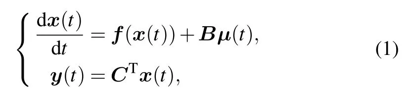
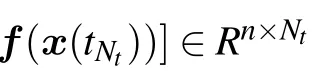
where x(t)∈Rn×1is the state variable with x(0)=x0,number n is the order of the system. f(x(t))is the nonlinear vector function, and μ(t)∈Rpis the input of the system with μ(0) = μ0. Variable y(t) ∈Rqis the system output, and B ∈Rn×pand C ∈Rn×qare the input and output matrices,respectively. In particular, these ordinary differential equations(ODEs)could arise from the discretization of partial differential equations (PDEs) based on numerical methods such as finite difference method (FDM) or finite element method(FEM).
2.1. Proper orthogonal decomposition based reduced model
We use the POD method to construct a reduced model for system (1). POD is a widely used data-driven modal decomposition method for obtaining low-complexity models.[8]Suppose we have collected a snapshot matrix Xsnap=[x(t1),...,x(tN)]∈Rn×N,where x(ti)represents the solution snapshot of system (1) at time ti. Then the k-dimensional(k ≪n)POD basis V for approximating state variable can be determined by taking the singular value decomposition(SVD)of snapshot matrix Xsnap,

where V ∈Rn×kand WT∈Rk×Nare real orthonormal matrices,and Σ ∈Rk×kis a diagonal matrix. Superscript symbol T represents the transpose of a matrix or a vector. With the constructed POD basis V, the state variable x(t) of system (1)can be approximated by
where a(t)∈Rkis a time-dependent coefficient vector. Substituting Eq.(3)into system(1)and then applying the Galerkin projection yield
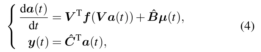
Unfortunately,the reduced system(4)usually is not able to evaluate VTf(V a(t)) efficiently. DEIM is an effective method to overcome the issue.[17]The DEIM approximates the nonlinear term of the system through the technique of interpolation. With the POD method,the f(x(t))in system(1)can be represented by
where U ∈Rn×mis the m-dimensional POD basis obtained by taking the SVD of the snapshot matrix of the nonlinear term,c(t)∈Rm×1is the time-dependent coefficient vector. Multiplying both sides of Eq.(5)by matrix PTand then solving for the coefficients vector c(t), we obtain the DEIM approximation

where P =[er1,...,erm]∈Rn×m,eri∈Rnis the ri-th column of identity matrix In∈Rn×n,and riis the interpolation index.In this expression,interpolation matrix P plays a crucial role for the approximation error and can be obtained by executing the greedy search algorithm provided in Ref.[17].
Substituting Eq.(6)into Eq.(4),we obtain
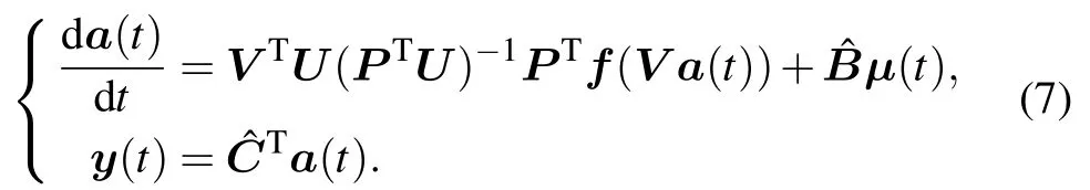
We call Eq.(7)the POD-DEIM reduced system. In(7), nonlinear term f(V a(t)) is only evaluated at the elements corresponding to the interpolation indices, and thereby the efficiency can be greatly improved.After obtaining the POD basis V,U and interpolation matrix P,matrix VTU(PTU)−1can be precomputed on the off-line stage. Here, matrix PTU ∈Rm×mis non-singular.
3. An improved interpolation method with linear approximation
As described above, for the DEIM method, only a few entries corresponding to the interpolation indices are selected to reconstruct the nonlinear function f(x(t)). This will inevitably lose the information contained in the unselected part.For this reason,an improved DEIM is presented by using linear truncation. We attempt to extract the information of the nonlinear function as much as possible before applying the DEIM approach,so as to reduce the error caused by interpolation.
We decompose the f(x(t))of system(1)as
where flin(x(t)) and fres(x(t)) represent the linear approximation term and its residual term,respectively. Instead of applying the DEIM approach to the nonlinear term f(x(t))directly,we only compute the DEIM approximation of the residual term fres(x(t)),
where Φ ∈Rn×mand S ∈Rn×mare the POD basis and the interpolation matrix that are calculated through the sampled data of the residual term {fres(x(t1)),...,fres(x(tN))}. Note that to calculate Φ and S, we need to first collect the snapshots of nonlinear function f(x(ti))and compute flin(x(ti)),and then obtain the sampled data fres(x(ti)) = f(x(ti))−flin(x(ti)),i=1,2,...,N.
With Eqs.(8)and(9),we have
Through retaining the linear approximation of the original nonlinear function, model (10) has more advantage than the classical DEIM method in obtaining an accurate approximation of f(x(t)),which has been shown by the error analysis in Subsection 3.3. In addition,considering the efficiency of the reduced system,flin(x(t))should allow for a low-cost storage and a fast evaluation.
3.1. Linear approximation based on Taylor series expansion
Obviously, the linear approximation term flin(x(t)) can be constructed by using Taylor series expansion. Based on Taylor series expansion,we have
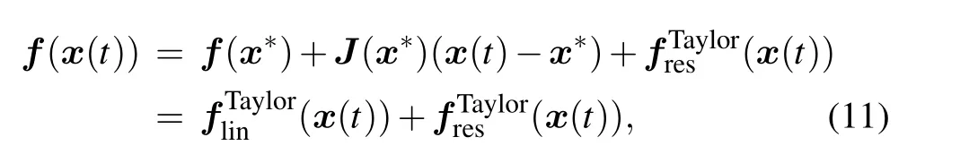


where all V ∈Rn×k, f(x∗) ∈Rn×1, J(x∗) ∈Rn×n, and VTΦ(STΦ)−1∈Rk×mare constant matrices and can be precomputed on the off-line stage. Hence, compared with the reduced system(7),system(13)also is efficient. For simplicity, we call model (12) Taylor-DEIM and system (13) PODTaylor-DEIM reduced system.
3.2. Linear approximation based on dynamic mode decomposition
As discussed above,we can construct the linear approximation term flin(x(t))with Taylor series expansion.However,this method has some limitations when the function f(x(t))is unknown or non-differentiable. Moreover, f(x(t))is a highdimensional nonlinear vector function,making it hard to compute the Jacobian matrix J(x∗) and select proper expansion points. Considering DEIM is a data-driven method, we construct another version of flin(x(t)) by employing DMD.[19]DMD is a data-driven and equation-free modal decomposition method. This method has recently gained increasing attention owing to its ability to reveal and quantify the dynamics of systems. In particular, DMD shows the marked improvement in the computational speed for evaluating the nonlinearity.[21,22]
We assume that {f(x(t1)),...,f(x(tN))} is a data sequence of the nonlinear term, where each f(x(ti)) =f(x(iΔt)), and Δt is a fixed sampling rate, N is the number of sampling. Because the DEIM method is itself a data-driven method, our method does not require additional sampling data. Let F0= [f(x(t1)),...,f(x(tN−1))], F1=[f(x(t2)),...,f(x(tN))], the linear operator can be approximated by
By means of the DMD procedure,the nonlinear function f(x(t))is approximated by

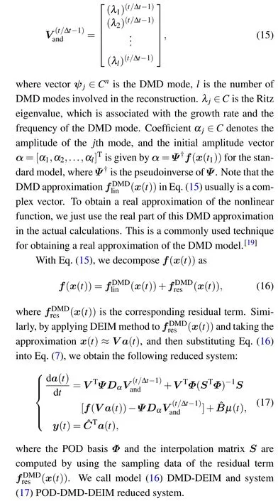

3.3. Error analysis
Next,we present an error analysis to show that model(10)has more advantage than model(6)in approximating the vector function f(x(t)). For simplicity, we sign f(x(t))=f,flin(x(t))=flin, fres(x(t))=fres, U(PTU)−1PT=P, and Φ(STΦ)−1ST=S. Let

To begin, consider a set of snapshots of residual term{fres(x(t1)),...,fres(x(tns)}∈Rn. Φ is the POD basis of the residual term fres, and we obtain Φ by solving minimization problem[8]

where Im∈Rm×mand In∈Rn×nare the identity matrices.Then,we have

Without loss of generality,assume that‖(In−ΦΦT)fres‖2=h, ‖(In−UUT)fres‖2=h+ε, where h,ε are non-negative constants,and ε =0 only for flin=0.
Next, we will analyze the error bounds of E0(t) and E1(t). From Eq.(18),we have
E0(t)=(In−P)(flin+fres).
Then,we have

According to Ref.[17],we have
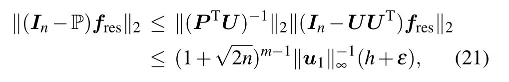
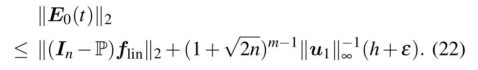
where u1is the first column of POD basis U,‖·‖∞represents the infinite norm of a vector. With inequalities(20)and(21),the error upper bound of E0(t)becomes
Similarly,from Eq.(18),we also have
‖E1(t)‖2=‖f −(flin+Sfres)‖2=‖(In−S)fres‖2.
Then,we have
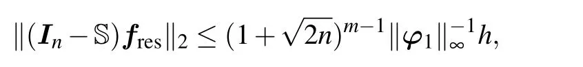
where φ1is the first column of POD basis Φ. Then the error upper bound of E1(t)can be obtained by
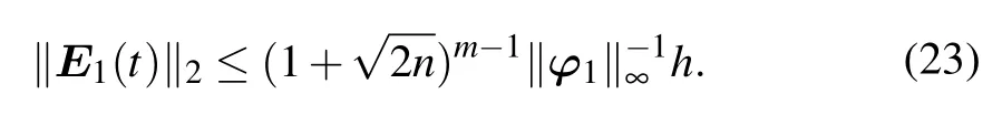
Referring to inequalities(22)and(23),we can notice that the error upper bounds of E0(t)and E1(t)are related to‖u1‖∞and‖φ1‖∞. Because POD is a data-driven method,we are not optimistic that the rigorous estimations of ‖u1‖∞or ‖φ1‖∞can be obtained mathematically. However, by comparing inequalities(22)and(23),it is evident that E1(t)has an advantage over E0(t)in obtaining a smaller error bound.
4. Modeling the error of the reduced system with neural networks
During constructing ROMs, some assumptions and approximations were employed,which inevitably leads to an error between the ROM and the original system. The errors of ROMs are crucial for the final resulting analysis. However,as the error analysis discussed in Subsection 3.3,DEIM is a datadriven method, and it is hard to estimate the error of DEIMrelated ROMs through theoretical analysis. To eliminate this drawback, we introduce a data-driven model to quantify the error of the POD-DEIM reduced system. The error model is constructed by using RBF neural networks[25]and can be computed cheaply. Once the error model has been built, we can correct the ROM with the prediction of the system error.
The state-space error of the reduced system can be expressed as
4.1. Optimization of the error model
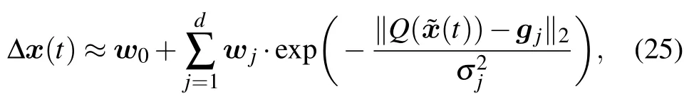
Two techniques are applied to enhance the efficiency of the error model (25). Firstly, the DEIM method is applied to select the model input,
where P1∈Rn×nqis an interpolation matrix obtained by DEIM.Since nq ≪n,the dimension of input variables of the error model can be reduced significantly.
Secondly,we choose the global and the local POD bases of state variable as the center vectors gjin Eq. (25). How to choose the center vectors is a crucial issue for RBF neural networks. Usually, it is difficult to make a reasonable choice of the center vectors from a large number of training samples. To overcome this issue,the POD technique was employed for the center vector selection in Ref. [30]. Specifically, the training samples were divided into many segments,and then the firstorder POD basis of each segment was chosen as one center vector. Because the number of segments is smaller than the number of training samples, the POD technique maintains a balance between the accuracy and the complexity of the RBF neural networks. However,they only use the local POD basis as the center vectors,not making use of the global information of training samples.Thus,in this work,both the global and the local POD bases of state variable are employed as the center vectors of RBF neural networks.
Suppose we have N training samples,then model(25)can be written in matrix form as
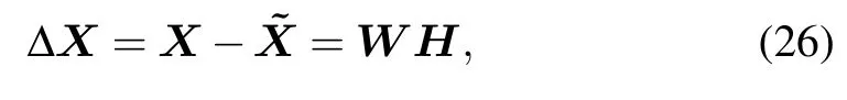
where
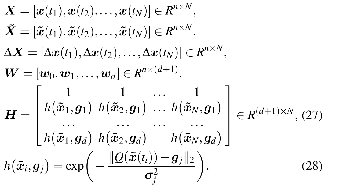
Note that equation (28) is a radial basis function, which is the activation function of the neural networks. Here,a combination of validation samples and heuristic algorithms can be used to determine the optimal structure and parameters of the neural networks,including the width value σjand the number of hidden neurons d.[25]
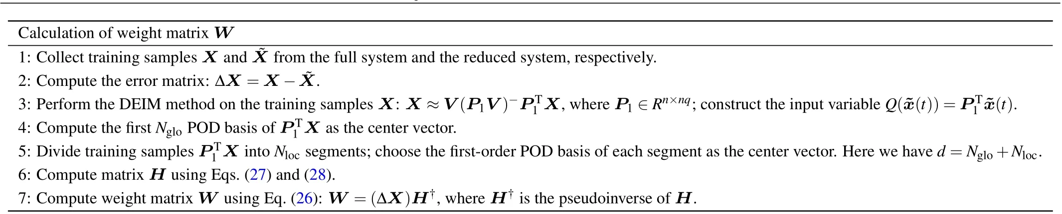
Calculation of weight matrix W 1: Collect training samples X and ˜X from the full system and the reduced system,respectively.2: Compute the error matrix: ΔX=X − ˜X.3: Perform the DEIM method on the training samples X: X ≈V(P1V)−PT1 X,where P1 ∈Rn×nq;construct the input variable Q(˜x(t))=PT1 ˜x(t).4: Compute the first Nglo POD basis of PT1 X as the center vector.5: Divide training samples PT1 X into Nloc segments;choose the first-order POD basis of each segment as the center vector. Here we have d=Nglo+Nloc.6: Compute matrix H using Eqs.(27)and(28).7: Compute weight matrix W using Eq.(26): W =(ΔX)H†,where H† is the pseudoinverse of H.
5. Results and discussion
Two examples are used to illustrate the effectiveness of the proposed model. The function ode15s in Matlab software is used to solve the full systems and the reduced systems. All the numerical simulations are performed on a desktop with Intel Core i7,3.4 Ghz,8 GB RAM,and software Matlab.
To check the accuracy of the model, the following relative errors are defined for nonlinear term f(x(t))and system output y(t):

5.1. Example 1: nonlinear transmission line circuit
We consider the nonlinear transmission line circuit system introduced in Refs. [4,5]. The circuit includes resistors,capacitors,and diodes. The resistors and capacitors have unit resistance and capacitance. The diode I-V characteristic is ic(v) = exp(40v)−1. Let x(t) = [x1(t),...,xn(t)]T, and xidescribes the voltage at node i at time t. The system input and output are the current source and the voltage at node 1, respectively, i.e., the input and output matrices are B =C =[1,0,...,0]T∈Rn×1. The system input µ(t)=exp(−t),t ∈[0,T].
The number of nodes of the original system is n=100.The total number of time steps is Nt=10000 (T =10, Δt =0.001). In this example,600 snapshots are uniformly selected from the original system in the interval [0,6] to construct the reduced systems. For the DMD-DEIM model, the number of DMD modes is fixed to 10. Figure 1 displays the relative error for approximating the nonlinear term of the system versus the dimension of the POD basis. The relative errors of Taylor-DEIM and DMD-DEIM are obviously smaller than those of DEIM method, suggesting that the linear approximation method in Section 3 can improve the accuracy of approximating the nonlinear term. Moreover, DMD-DEIM almost has the same accuracy as Taylor-DEIM when the dimension of POD basis m ≤5. However, the DMD-DEIM gradually approaches the DEIM as the dimension of POD basis increases. The reason is that the performance of DMD-DEIM is influenced by the linear approximation term flin(x(t))and the residual term fres(x(t)), and the POD basis and interpolation matrix of the residual term are different from those of the nonlinear term. For comparison,figure 1 also gives the results of Taylor-POD and DMD-POD. Here, Taylor-POD and DMD-POD represent the models that we replace DEIM with the POD method to approximate the residual term. Because the DEIM method almost has the same performance as the POD method in approximating the residual term, the relative errors of Taylor-DEIM and DMD-DEIM are close to those of Taylor-POD and DMD-POD,respectively.
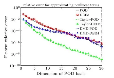
Fig.1. Relative error for approximating nonlinear term in Example 1.
Figure 2 presents the results of various reduced systems of order k=5, where the system outputs are shown in Fig.2(a)and the corresponding L1-norm relative errors computed by Eq.(29)are given in Fig.2(b). Without loss of generality,for all the reduced systems,we set the dimension of POD basis for state variable(k)and nonlinear term(m)the same,i.e.,k=m.In Fig.2(a), all the outputs of the reduced systems match the output of the full system well. However,it is clear that the relative errors of POD-Taylor-DEIM and POD-DMD-DEIM are much smaller than that of POD-DEIM in Fig.2(b).
Figure 3 compares the relative errors of the outputs between POD-DEIM reduced system and POD-DEIM-RBF reduced system for order k=5. Here,POD-DEIM-RBF represents the POD-DEIM reduced system with the error prediction model constructed by RBF neural networks. For error prediction model,the center vectors consist of 10 global POD bases and 20 local POD bases, the dimension of model input is 30,and width value σj=1. The fact that POD-DEIM-RBF performs better than POD-DEIM confirms the effectiveness of the error prediction model introduced in Section 4.
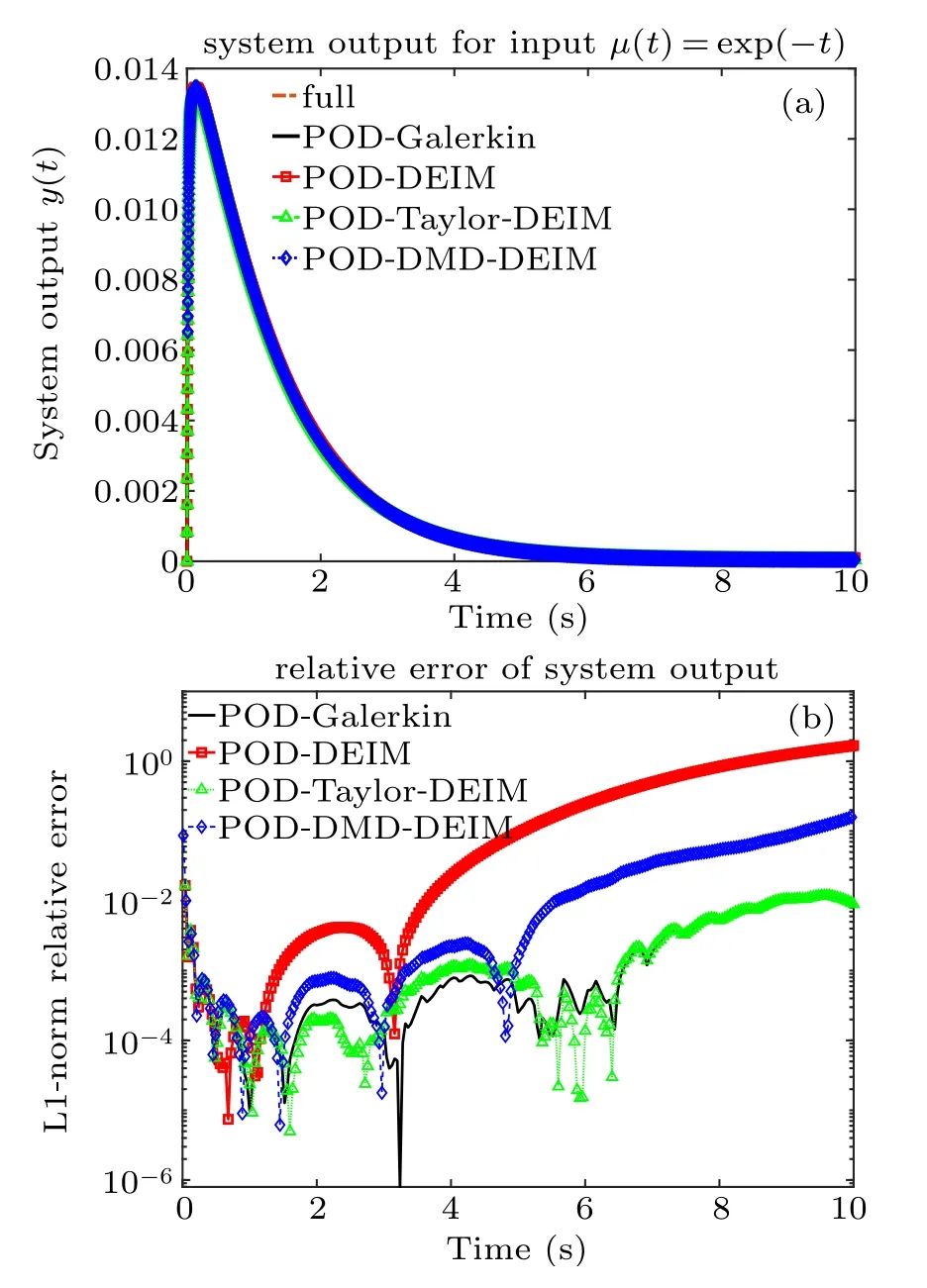
Fig.2. Example 1: (a) System outputs of various reduced systems of order k=5. (b)Relative error of the system output.
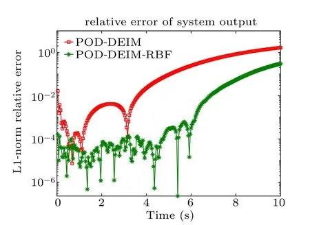
Fig.3. The relative error of the system output comparison between PODDEIM and POD-DEIM-RBF for Example 1, the order of reduced system k=5.
5.2. Example 2: Burgers’equation
Next, we consider one-dimensional Burgers’ equation with the following initial-boundary conditions:[6]
where
The dimension of the full model n=1000,L=100,xi=iΔx,Δx=L/n,T =60,Δt=0.01.For this test case,the POD basis is constructed from 600 snapshots obtained from the solutions of the full system at equally spaced time steps in the interval[0,T].
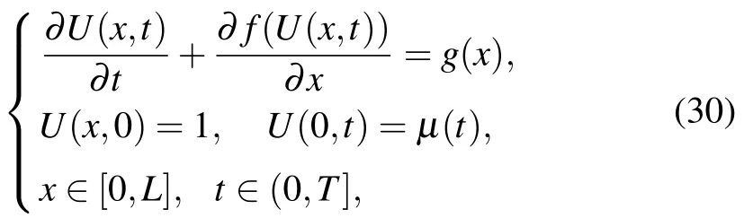
Figure 4 compares the abilities of different methods to approximate the nonlinear term of the system. It is apparent that Taylor-DEIM and DMD-DEIM are more accurate than DEIM.Similarly,Taylor-POD and DMD-POD are more accurate than POD.For DMD-POD and DMD-DEIM,the number of DMD modes is fixed to 100.Figure 5 shows the reconstructions of state variables when the orders of the reduced systems are k=50. Generally,the results in Fig.5 are consistent with those in Fig.4. As shown in Fig.5, the curves of PODGalerkin, POD-Taylor-DEIM, and POD-DMD-DEIM match the curves of the full system better than those of POD-DEIM.

Fig.4. Relative error for approximating nonlinear term in Example 2.
Figure 6 reports the results of POD-DEIM-RBF reduced system. For POD-DEIM-RBF, the center vectors of the error prediction model consist of 50 global POD bases and 10 local POD bases, the dimension of model input is 50, and width value σj=10. As shown in Fig.6(a), the curves of POD-DEIM-RBF match the curves of the full system better than those of POD-DEIM.The corresponding relative error of the system output is shown in Fig.6(b),where the relative error of POD-DEIM-RBF is smaller than that of POD-DEIM.Here, we assume that the system output y(t) = CT¯U(x,t),where C = [1,...,1]T. Moreover, it is worth mentioning that the error prediction model can be extended to other lowfidelity reduced systems. For example, figure 6(b) also provides the simulation results of POD-Galerkin-RBF reduced system (using POD-Galerkin to replace the POD-DEIM in POD-DEIM-RBF). Similarly, POD-Galerkin-RBF has superior performance to POD-Galerkin.
Fig.5. Example 2: reduced systems of order k=50. (a)POD-Galerkin. (b)POD-DEIM.(c)POD-Taylor-DEIM.(d)POD-DMD-DEIM.
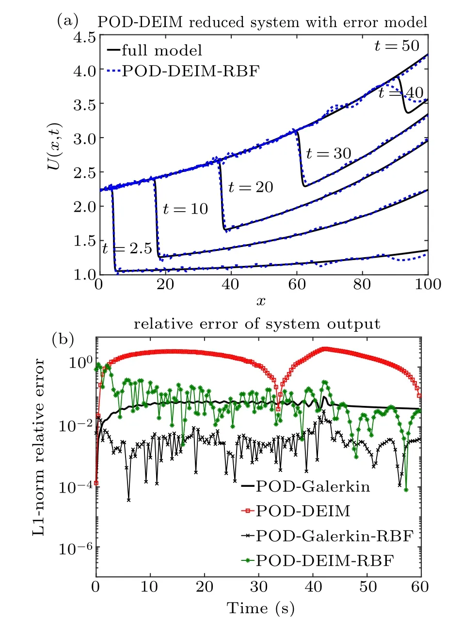
Fig.6. Example 2: reduced systems of order k=50. (a) The PODDEIM reduced system with error prediction model. (b) Relative error of system output.
Table 1 lists the average CPU time for constructing(offline) and solving (on-line) the reduced systems. The PODTaylor-DEIM almost has the same off-line and on-line CPU time as the POD-DEIM. However, compared with PODDEIM, POD-DMD-DEIM takes more CPU time both on the off-line and the on-line stages. This is because the PODDMD-DEIM needs to compute the DMD approximation of the nonlinear term. In addition, the POD-DEIM-RBF costs more CPU time than the POD-DEIM both for the off-line stage and the on-line stage. The reason is that the PODDEIM-RBF needs to construct the error remedy model on the off-line stage. For the on-line stage, POD-DEIM-RBF executes the error remedy model to predict the state-space error of POD-DEIM reduced system. However, in terms of accuracy,POD-DMD-DEIM and POD-DEIM-RBF are competitive with POD-DEIM in this example.

Table 1. The average off-line and on-line CPU time(second)of various reduced systems.
6. Conclusions
This work introduced an improved DEIM method for nonlinear model reduction. The improved DEIM first constructed a linear approximation for the nonlinear term of the system, and then evaluated the residual between the linear approximation and the nonlinear term by using the standard DEIM. The line approximation term was constructed by the linear Taylor’s expansion and the data-driven method,respectively. The error analysis was also provided to show the effectiveness of the proposed method.
Moreover, an error prediction model was introduced for the low-fidelity reduced models based on the RBF neural networks. To enhance the computational efficiency, the DEIM was applied to extract the input of the neural networks,and the global and the local POD bases of state variables were chosen as the center vectors of the neural networks. At last,our proposed method was tested on nonlinear transmission line circuit system and one-dimensional Burgers’equation. The example results showed that our approach is efficient and can significantly improve the accuracy of the low-fidelity reduced system.
- Chinese Physics B的其它文章
- Transport property of inhomogeneous strained graphene∗
- Beam steering characteristics in high-power quantum-cascade lasers emitting at ~4.6µm∗
- Multi-scale molecular dynamics simulations and applications on mechanosensitive proteins of integrins∗
- Enhanced spin-orbit torque efficiency in Pt100−xNix alloy based magnetic bilayer∗
- Soliton interactions and asymptotic state analysis in a discrete nonlocal nonlinear self-dual network equation of reverse-space type∗
- Discontinuous event-trigger scheme for global stabilization of state-dependent switching neural networks with communication delay∗