Periodic Variation Solutions and Tori like Solutions for Stochastic Hamiltonian Systems

ZHU Jun(朱俊),LI Ze(黎泽)

(School of Mathematics and Statistics,Ningbo University,Ningbo 315211,China)

Abstract: In this paper,we study recurrence phenomenon for Hamiltonian systems perturbed by noises,especially path-wise random periodic variation solution (RPVS)and invariant tori like solution.Concretely speaking,for linear Schrödinger equations,we completely clarify when RPVS exists,and for nearly integrable Hamiltonian systems perturbed by noises we prove that the existence of invariant tori like solutions is related to the involution property of multi component driven Hamiltonian functions.

Key words: Random system;Hamiltonian system;Recurrence phenomenon;Invariant tori

1.Introduction

We first consider finite dimensional random dynamical systems.LetMbe a 2ddimensional symplectic manifold with symplectic form m.Given a Hamiltonian functionHonM,the associated Hamiltonian vector field is denoted byXH.Given a filtered probability space(Ω,F,P),letZtbe an Rl-valued driving semi-martingale,Y0∈F0be anM-valued random variable,and{Hα}lα=0be Hamiltonian functions onM.We will study the following type stochastic differential equations which may be seen as the analogies of Hamiltonian systems of the deterministic case:

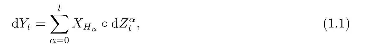
where◦refers to the Stratonovich integral and(1.1)is understood in the sense of the integral equation with initial dataY0.Moreover,for simplicity we write dt=dZ0tin (1.1)and in the following.

Let’s first consider the caseM=T∗Td,where Td=Rd/2πZddenotes thed-dimensional torus.In the perturbation theory,one considers the Hamiltonian functions defined inT∗Td,which can be viewed as Td×Rd,of the following form

where (p,q)∈Rd×Tdis the action and angle variables respectively.IfH1= 0,the Hamiltonian system associated with (1.2)is integrable.IfH1(p,q)is a small perturbation in some sense,the Hamiltonian system corresponding to (1.2)is called nearly integrable.The classic celebrated KAM theorem[2]states that the invariant tori persists under the perturbation with suitable non-degenerate conditions.The KAM theory in the deterministic case is a fundamental result of Hamiltonian systems,and it has many significant and wide applications to various problems,for instance celestial mechanics,symplectic algorithms[3,7],Anderson localization etc.In the stochastic case,few results are known.Let (Ω,F,P,{θt}t∈R)denote the canonical metric dynamical system describing R1-valued Brownian motion{Bt}t∈R.Let us begin with the toy model problem:

whereN0,N1only depend onp,∇Nidenotes the gradient field generated byNi,andJdenotes the standard complex structure in R2d.The solution of (1.3)can be written as

This can be seen as the stochastic version of integrable systems.Now,assume that for someZd,∂piN0(p∗)=2πki/Tfor alli=1,··· ,d,then it is easy to see

with (ξ,ζ)=(0,··· ,0,∂p1N1(p∗)BT(ω),··· ,∂pdN1(p∗)BT(ω))for all (t,ω)∈R×Ω,and as a random dynamical system[1]there holds

whereφ(t,ω)(p,q)denotes the solution of (1.3)with initial data (p,q).

Inspired by(1.5),(1.6),we introduce the notion of periodic variation solutions as follows:

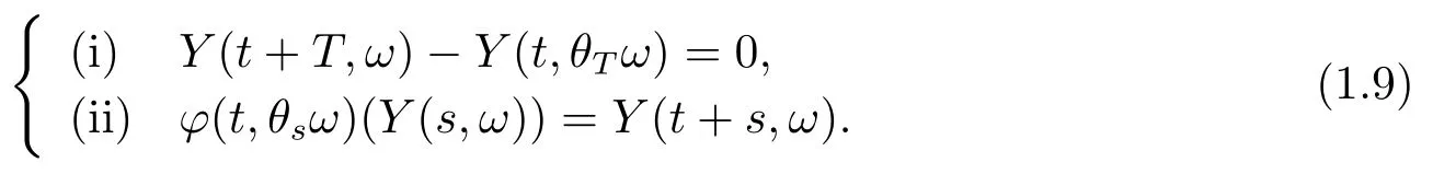
Definition 1.1LetMbe a finite or infinite dimensional linear space or a smooth manifold embedded into Euclidean spaces.Letφ:Λ×Ω×M →Mbe the mapping which defines a measurable random dynamical system on the measurable space(M,B)over a metric random dynamical system (Ω,F,P,(θt)t∈Λ).We sayY(t,ω)is a random periodic variation solution (RPVS)withF0measurable initial dataY(0,ω)if there exists someT >0 and anM-valued (whenMis a linear space)or RN-valued (whenMis a manifold)random functionξ:ω ∈Ω →Morξ:ω ∈Ω →RNsuch that for allt ∈Λ,ω ∈Ω,there holds

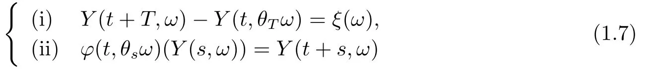
where (i)in (1.7)holds in the Euclidean space RNifMis a manifold embedded into RN.

If the random dynamical system is a two parameter stochastic flowφ:I×I×Ω×M →M,(1.7)is replaced by

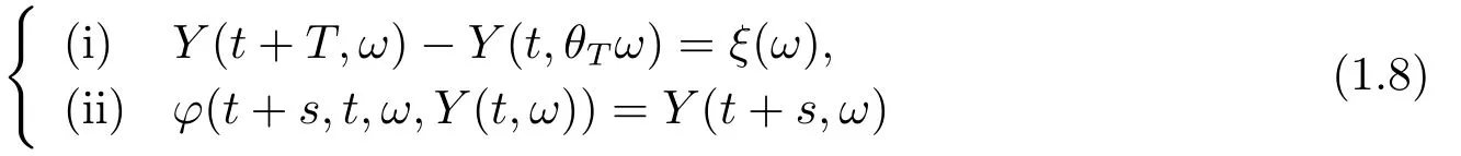
for anyt,s ∈I,ω ∈Ω.

If we requireξ=0 in(i)of(1.7),then solutions satisfying(1.7)are called random periodic solutions (RPS),i.e.,

See the works of ZHAO,et al.[13]and FENG,et al.[6]for existence of RPS of contraction systems and dissipative systems.

The other widely used notion of periodic solutions is the periodic Markov process solution:We say the solution of a stochastic equation is a periodic homogeneous Markov process solution if it is an Rmvalued homogeneous Markov process and the joint distribution P(ut1∈A1,··· ,utn ∈An)satisfies

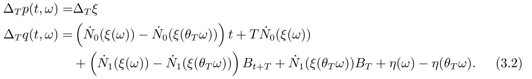
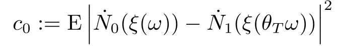
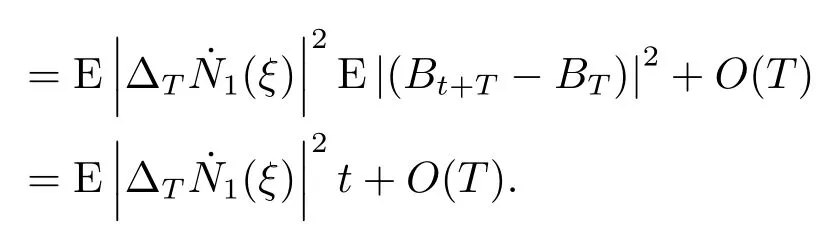
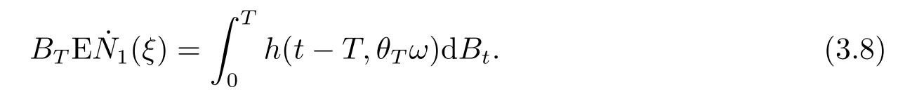
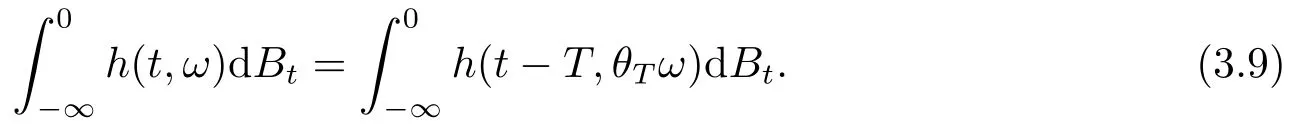
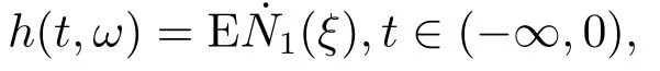
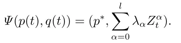
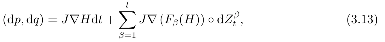
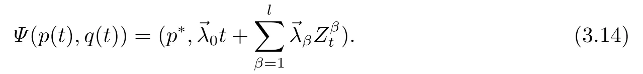
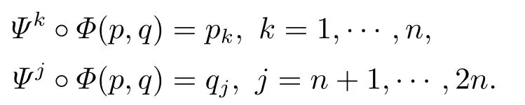
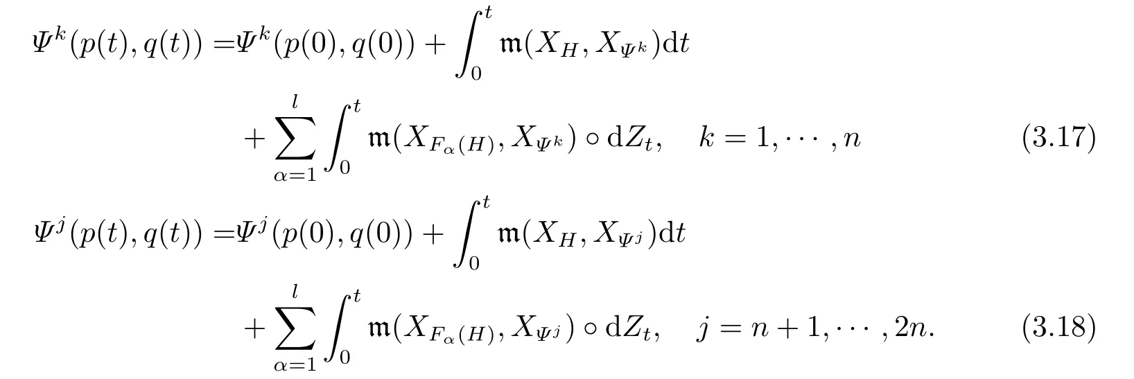
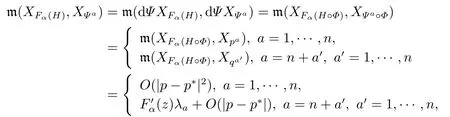
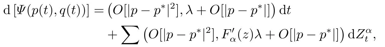
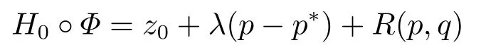
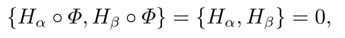
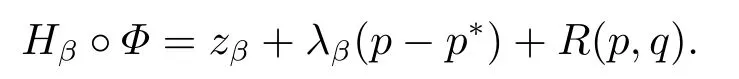
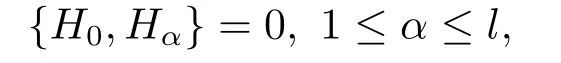
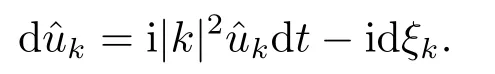
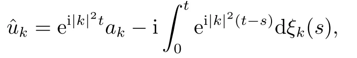
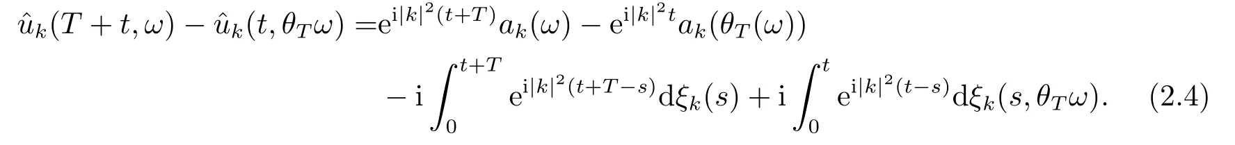
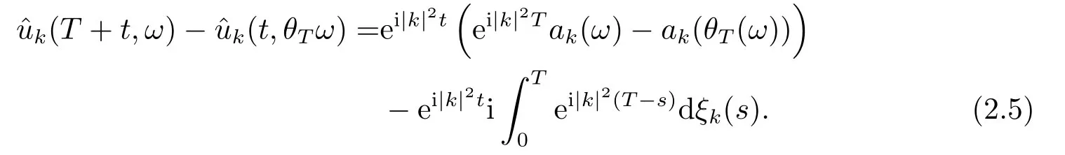
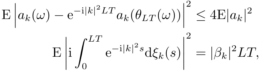
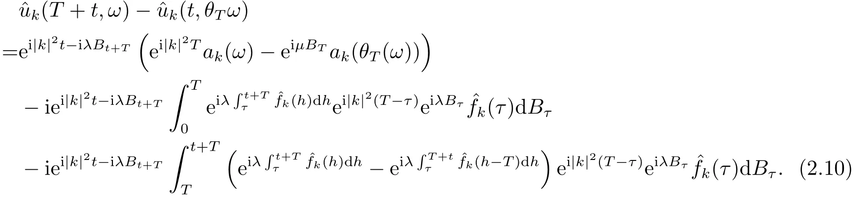
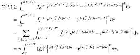
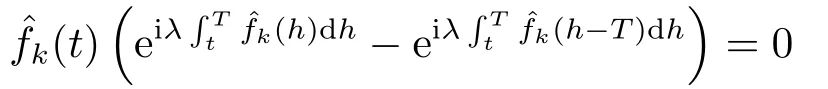
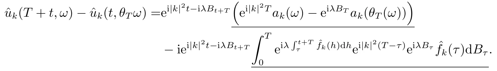
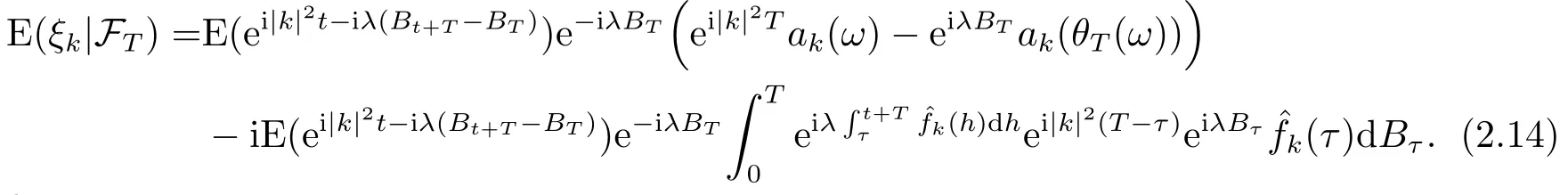
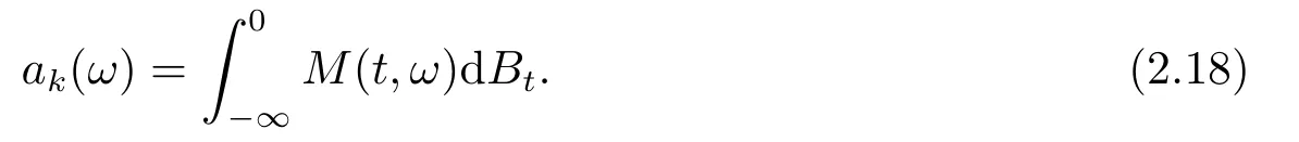
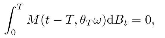
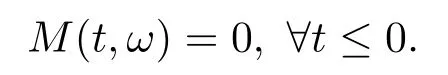
for someT >0 and all 0≤t1<···

We summarize the existence/non-existence of RPS and RPVS for (1.3)in the following lemma.It is somewhat casual,and the precise statement can be found in Section 3.

Proposition 1.1(1.3)has no random periodic solutions except for some trivial cases(See Proposition 3.1).ForF0measurable initial data (p(0),q(0))= (ξ,η),the solution of(1.3)is a random periodic variation solution iff{∇Ni(ξ)}i=0,1are deterministic.

In general,if the frequencies{∂piN0(p∗)}di=1are rationally independent,the solution of(1.3)is invariant tori like:

where{Yj(t,ω)}dj=1are RPVSs.

If there is essentially only one driving Hamiltonian in (1.1),i.e.,Hα=Fα(H)for allα= 0,··· ,l,it is easy to apply the classic KAM theorem to obtain random invariant tori like solutions in the stochastic case.Generally multi driving Hamiltonian functions may lead to non-existence of invariant tori.For the special cased= 1,we will see there exists a neat result:

Proposition 1.2Letd=1.LetH0be a Hamiltonian function on R×T which gives rise to a small analytic perturbation of integrable systems.Let{Hα}lα=1be analytic functions ofp,q ∈C2.If the driving Hamiltonian functions satisfy

then under reasonable non-degenerate assumptions,(1.1)has random invariant tori.See Proposition 3.2 for the precise statement.

In a summary for SODEs,we remark that(i)Random periodic solutions generally do not exist for Hamiltonian type equations;(ii)The existence of random periodic variation solutions and invariant tori depends heavily on the involution property of the driving Hamiltonian functions.

Let’s consider infinite dimensional random dynamical systems.Let(Ω,F,(Ft)t∈R,P,(θt)t∈Λ)be the canonical complete filtered Wiener space endowed with filtrationFts:=σ{Br1−Br2:s ≤r1,r2≤t}.DenoteandLet{ζj(t)}j∈Zbe a sequence of independent R-valued standard Brownian motions ont ∈R associated to the filtration(Ft)t∈R.LetΦ:L2(Td;C)→L2(Td;C)be a linear bounded operator withQ=ΦΦ∗being a finite trace operator inL2(Td;C).Lettingbe the orthonormal basis forL2(Td;C),we define the processWto be

It is easy to see the series (1.11)converges inL2(Ω×Td;C)and almost surely inL2(Td;C).This process is a special case ofQ-cylindrical Wiener process withQ=ΦΦ∗.

Theorem 1.1(i)IfΦ0,then the linear stochastic Schrödinger equation with addictive noise

has no RPVS.

(ii)Let us consider the linear stochastic Schrödinger equation with combined noise:

whereλ ∈R,fis a real valued function which is periodic int,f(t+T1)=f(t),and smooth inx ∈Td.Thenuis an RPVS withF0measurable initial datau0∈L2(Ω,L2x)for (1.12)if only iff=0 andu=0.

In the following,we denote ∆Tu(t,w)=u(t+T,w)−u(t,θTw).

2.Linear SPDEs

We divide the proof of Theorem 1.1 into two propositions.Let{ek}k∈Zdbe the eigenfunctions of ∆in Tdsuch that ∆ek=−|k|2ek,andπkdenote the projection onto span{ek}.We getf:Ω →L2xis (F,B(L2x))measurable iffπkfis (F,B(C))measurable for allk ∈Zd.And similar results hold withFreplaced byFts,FtandFtas well.These facts will be used widely in this section without emphasis.

Proposition 2.1Assume that the operatorΦ0 in (1.11).The linear stochastic Schrödinger equation with addictive noise

has no RPVS.

ProofDefine

then we haveE|ξk(t,ω)|2=|t|β2kwhere{βk}are defined by

Applying the Fourier transform to (2.1)gives

The solution is an Ornstein-Uhlenbeck process

whereak=(u0,ek),k ∈Zd.Thus we have

And by change of variables,(2.4)reduces to

Thus,ifuis a random periodic variation solution,then there holds

By iteration of (2.6),there holds

Since we have by be Cauchy-Schwartz inequality and the Itisometry formula that

the contradiction follows ifβk0 by lettingL →∞.Therefore,βk=0 for allk ∈Zd,which leads toΦ= 0,since{}j∈Zand{ek}k∈Zdare complete bases.Hence,no random periodic variation solution exists ifΦ0 .

Proposition 2.2Let us consider the linear stochastic Schrödinger equation with combined noise:

whereλ ∈R,fis a real valued function which is periodic int,f(t+T1)=f(t),and smooth inx ∈Td.Thenuis an RPVS withF0measurable initial datau0∈L2(Ω,L2x)for (2.8)if only iff=0 andu=0.

ProofSince (2.8)is non-autonomous,for RPVS,we use the definition in (1.8).Let us choose the eigenfunctions{ek}for Laplacian to be real valued functions,The solution is written as

whereak=(u0,ek),k ∈Zd.Then one has by change of variables that

Now,we prove RPVS exists ifff=0 andu=0.Assume thatuis an RPVS,i.e.∆Tu(t)=ξfor someF-measurable random variableξand allt ≥0.

Step 1 Taking the covariance of both sides of (2.10),we obtain by the Itô isometry formula and the Cauchy-Schwartz inequality that

for allt ≥0.Sincefis real valued and we have taken the orthogonal basis to be real functions,we see{}are real fork ∈Zd.Then byf(t+T1)=f(t)for allt ≥0,one has

forn ∈Z.Thus (2.11),(2.12)show

where in the last line we applied the periodicity off,(2.12)and change of variables.Thus,lettingn →∞,we get

which by the periodicity offfurther shows that

holds for allt ≥0.Assume thatis not identically zero.Let(t1,t2)be any interval contained in((0,∞)),then,choosing|t1−t2|to be sufficiently small,we have fort ∈(t1,t2)

for someL ∈Z which depends ont1,t2and is independent oft ∈(t1,t2).Taking derivatives tot ∈(t1,t2)yieldsfort ∈(t1,t2).

Back to (2.10),we see,for allt ≥0,

Recall ∆Tu=ξ.DenoteSinceu0isF0measurable,the underline parts areFTmeasurable.Taking conditional expectation E(·|FT),by the independence ofBt+T −BTandFT,we have

Thus since

by taking covariance of (2.14)and the Itô formula,we get that

which ast →∞yields E(ξk|FT)=0,a.s.

Inserting this to (2.14)shows

Then by iteration we obtain for allt ≥0

where we chosetj:=LT −(j+1)Tand applied the fact thatTis a period off.Then by the Itformula,

Therefore,by lettingL →∞,we see there exists no RPVS iffis nontrivial.

Step 2 Now,it remains to consider the degenerate case whenf ≡0.In this case,(2.10)reduces to

which combined withθ∗TP=P gives

where in the second equality we usedBT −B0is independent ofF0andu0isF0adapted.

LettingL →∞,by (2.16),we have

SinceF0:=σ{Bt −Bs:s,t ≤0},u0isF0measurable and belongs toL2(Ω;L2x),we obtain by(2.17)and the representation theorem for square integrable random variables (see Theorem 1.1.3 in [11])that there exists a unique adapted processMt ∈L2((−∞,0)×Ω)such that

Thus,by the same reason as (2.16),we see from (2.15)that

Then,applying (2.18),we arrive at

which by change of variables gives

SinceM(t −T,θTω)andM(t,ω)areFtadapted and belong toL2((−∞,0)×Ω),by the Itô formula,(2.19)shows

Taking conditional expectation of both sides of (2.15)w.r.t,FT0gives

which combined with (2.18)shows

However,sinceFT0is independent ofF0,we see E(ak|FT0)=E(ak)=0.

Thus (2.21)shows

which by the Itô formula further yields

SinceθTis invertible,taking(2.22)as the starting point and doing iteration by(2.20)illustrate that

Therefore,we conclude from (2.18)that

3.Finite Dimensional Case

In this section,we prove the results stated in Section 1 for SODEs.

Proposition 3.1LetN0,N1beC1bounded functions ofp ∈Rd.Consider the SODE for (p,q)∈Rd×Td:

Then we have

1)(p,q)is RPVS if and only if∇pN0(ξ),∇pN1(ξ)are independent ofω;

2)(p,q)is RPS if and only ifwithandη,ξare deterministic.

ProofStep 1 The solution for (3.1)is given by

The covariance of (3.2)is of orderc0t2ast →∞,ifc0defined by

does not vanish.If (p,q)is an RPVS,then the covariance of ∆Tq(t,ω)is identical w.r.t.t ≥0.Thusc0= 0.SinceξisF0measurable,isFTmeasurable.ThenBt+T −BTis independent ofHence there holds

Thus byc0= 0,the covariance of (3.2)is of orderc1tast →∞ifc1:=is not zero.Hence,c1=0 as well.Now we summarize that if (p,q)is an RPVS then

(3.3)impliesNi(ξ)is independent ofωby similar arguments in Section 2.In fact,the representation theorem of square random variables show

forMi ∈L2((−∞,0)×Ω)because(ξ)∈L2(Ω)isF0measurable fori= 0,1.Inserting(3.4)into (3.3)yields

Then the Itô formula shows

Therefore,we arrive at

namely,they are independent ofω.

Step 2 If we assume furthermore that (p,q)is an RPS,then by (3.5)and (3.2),for someZdthere holds

Similar arguments as Step 1 show that(3.6)impliesξis deterministic.And we seeTE(ξ)=by applying mathematical expectation to (3.7)sinceθ∗P = P.Writingη= E(η)+for someh ∈L2((−∞,0)×Ω),taking conditional expectation of (3.7)w.r.t.FT0,one obtains

And taking conditional expectation of (3.7)w.r.t.F0gives

Sincethe Itformula with (3.8)shows

By (3.10)and (3.11),we have

which belongs toL2((−∞,0)×Ω)if and only if E(ξ)=0.Hence,we have deduced

Therefore,by Step 1,we conclude that (p,q)is an RPS if and only if

We have several examples:

Example 3.1Letd= 2,N0(p)=f(p1),N1(p)=g(p1),then (p0,q0)= (c1,ϕ,ψ1,ψ2),wherec1is deterministic andϕ,ψ1,ψ2areF0adapted random variables,evolves to an RPVS.It is an RPS iffψ1,ψ2are deterministic.

Givenϱ>0.p∗∈Rd,define the setDp∗,ϱ={(p,q)∈C2d:|p −p∗|≤ϱ,|ℑq|≤ϱ},whereℑq= (ℑq1,··· ,ℑqd).Let Ap∗,ϱbe the set of complex valued continuous functions onDp∗,ϱwhich are analytic functions in the interior,2π-periodic inq(i.e.f(p,q+2π)=f(p,q),∀f ∈Ap∗,ϱ)and real valued for (p,q)∈R2d.

Proposition 3.2LetH0be a Hamiltonian function of the formH0=N(p)+ϵ(p,q)withN,∈Ap∗,ϱ.Denote

Assume that (Bij)is a non-singulard×dmatrix andsatisfies the Diophantine condition,i.e.there exists a positive constantγsuch thatdefined by

•Consider the stochastic ODE (1.1)in R1×T with Hamiltonian functions{Hα}0≤α≤lwhich satisfy

And assume that{Hα}lα=1are analytic functions inDϱ,p∗and continuous to the boundary as well.Then there exists a constantϵ0>0 such that for givenϵ ∈[0,ϵ0] there exists a symplectic transformΨ:Dϱ′,p∗→Dϱ,p∗and solution (p(t),q(t))to (1.1)satisfying

for someconstantsλα ∈R,α=1,··· ,l,andλ0=∂pN(p∗).

•Letd ≥1.Consider the stochastic ODE (1.1)in Rd×Tdwith Hamiltonian functionsH0(p,q)=N(p)+(p,q)and{Fβ(H0)}1≤β≤l:

where{Fβ}are smooth functions.Then there exists a constantϵ0>0 such that for givenϵ ∈[0,ϵ0] there exists a symplectic transformΨ:Dϱ′,p∗→Dϱ,p∗satisfying

ProofStep 1 Letλ=∇N(p∗)be the unperturbed frequency.By the classic KAM theorem,there exists a symplectic differmorphismsuch that

in(p,q)for somez ∈R and an analytic functionR(·,·)which is of the order|p−p∗|2.

We will frequently use the following identity

DenoteΨ=(Ψ1,··· ,Ψ2d)the inverse ofΦ,then

Assume that (p(t),q(t))solve (3.13),then by Itô’s formula

By (3.16)and the factΦis a symplectic differmorphism,we get

where in the last line we applied the Taylor expansion toFαatzand used (3.15)to expandH ◦Φ.

Thus (3.17),(3.18)show

which implies that (3.14)is a solution.

Step 2 It remains to prove the left S1×R1case.Applying (3.15)toH0gives the expansion

for some symplectic differmorphismΦ,z0∈R,λ=H′0(p∗),andRis of order|p −p∗|2.SinceΦkeeps the symplectic form,

where we applied (3.12)in the last line.Therefore,we arrive at

for allβ=0,...,l.Denote=Hβ ◦Φ.Then one sees

Then,comparing the coefficients of zero and one order of|p −p∗|,(3.19)gives

Sinceλ0,A0(q)andA1(q)are constants.Thus (3.20)shows the symplectic transformΦtransforms all{Hα}into the canonical form

Then the same argument in Step 1 gives the desired result.