
GLOBAL WEAK SOLUTIONS TO THE α-MODEL REGULARIZATION FOR 3D COMPRESSIBLE EULER-POISSON EQUATIONS∗
2021-06-17 13:58任亚伯
关键词:亚伯
(任亚伯)
Faculty of Science,Beijing University of Technology,Beijing 100124,China
E-mail:ryb2018@emails.bjut.edu.cn
Boling GUO(郭柏灵)
Institute of Applied Physics and Computational Mathematics,P.O.Box 8009,Beijing 100088,China
E-mail:gbl@iapcm.ac.cn
Shu WANG(王术)
Faculty of Science,Beijing University of Technology,Beijing 100124,China
E-mail:wangshu@bjut.edu.cn
AbstractGlobal in time weak solutions to the α-model regularization for the three dimensional Euler-Poisson equations are considered in this paper.We prove the existence of global weak solutions to α-model regularization for the three dimension compressible Euler-Poisson equations by using the Fadeo-Galerkin method and the compactness arguments on the condition that the adiabatic constant satisfies γ>
Key wordsGlobal weak solutions;α-model regularization for Euler-Poisson equations;Faedo-Galerkin method
1 Introduction
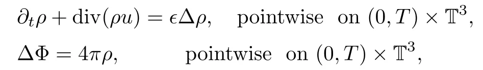
The motion of a compressible isentropic perfect fluid with self-gravitation is modeled by the Euler-Poisson equations in three space dimensions:

where t≥0,x∈T3,ρ,u=(u1,u2,u3),P(ρ)and Φ represent the fluid density,velocity,pressure and gravitational potential,respectively.We assume that the pressure function P(ρ)satisfies the usual γ-law,

for some γ>1.
In this paper,we consider the global weak solutions to Euler-Poisson equations with a viscosity term:
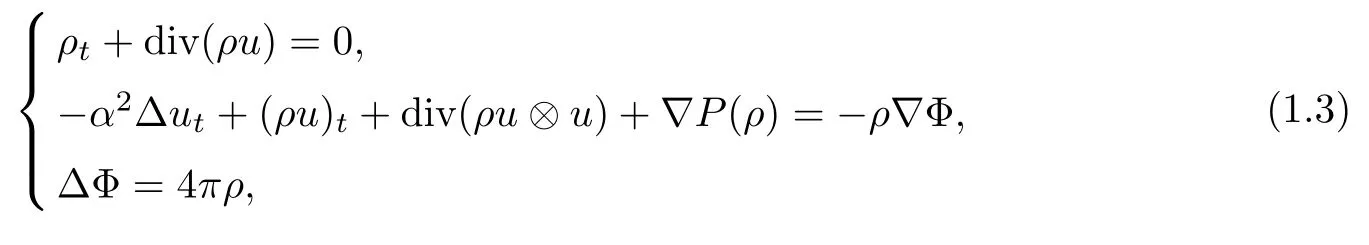
with the initial conditions

Equation(1.3)is also known as the α-model regularization for the Euler-Poisson equations.The term−α2Δutis a small perturbation,representing some kind of friction.The term on the right hand side of the second equation in(1.3)describes the internal force of gradient vector field produced by potential function,which can be uniquely solved by the Poisson equation(1.3)3.The potential function is given by

where G(x,y)denotes the Green’s function of the Poisson part.
In particular,if without the term−α2Δut,the equations(1.3)will be reduced to the Euler-Poisson equations.This describes the motion of a compressible isentropic perfect fluid with selfgravitation in three space dimensions(compare[11]).T.Luo and J.Smoller proved in[14]that the non-linear dynamical stability of compressible Euler-Poisson equations with perturbations have the same total mass and symmetry as the rotating star solution.A rigorous mathematical theory for rotating stars of compressible fluids was initiated by Auchmuty and Besls[15]in 1971.The existence and properties of rotating star solutions were obtained by Auchmuty and Besls[15],Auchmuty[13],Caffarelli and Friedman[16],Friedman and Turkington[17,25],Li,Chami-llo and Li[19],and Luo and Smoller[20].In[24],McCann proved an existence result for rotating binary stars.In contrast,the existence and properties of stationary non-rotating star solutions is classical(see[11]).
In this paper,we prove the existence of weak solutions to(1.3)by using the Faedo-Galerkin method(see[4,23]).When we deduce the energy estimates and B-D entropy,the estimates will depend on the index∊,δ and η,so we need to be very careful as we deduce these estimates because we need to tend the∊,η,δ to zero step by step later in the proof of the main theorem.In addition,B-D entropy can also be applied to other equations;for more details,the reader can refer to[12,18,21,22]and references therein.
1.1 Formulation of the weak solutions and main result
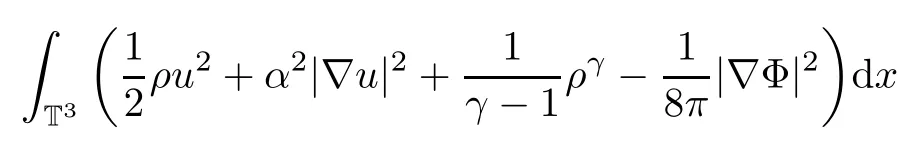
For the smooth solutions(ρ,u,Φ(ρ)),multiplying equation(1.3)2and integrating by parts,we can deduce the following energy inequality:

However,the above energy estimate is not enough to prove the stability of the weak solutions(ρ,u,Φ(ρ))of(1.3).We will obtain the following B-D entropy estimate,which was first introduced by Bresh-Desjardins in[10]:

where C is bounded by the initial energy.Thus the initial data should satisfy the following:

Definition 1.1We will say that(ρ,u,Φ)is the finite energy weak solution of problems(1.3)and(1.4)if the following is satisfied:
1.ρ,u belong to the classes

2.The equations(1.3)1–(1.3)2hold in the sense of D′((0,T)×T3),(1.3)3holds a.e.for(t,x)∈((0,T)×T3);
3.(1.4)holds in D′(T3);
4.(1.6)and(1.7)hold for almost every t∈[0,T].
NotationsThroughout this paper,C denotes a generic positive constant which may depend on the initial data or some other constant independently of the indexes∊,η,δ and r0,and C(·)>0 means that the constant C depends particularly on the parameters in the bracket.
We now state our main results.
Theorem 1.2Letting γ>and letting the initial data be satisfied by(1.8),for any time T there exists a weak solution(ρ,u,Φ)to(1.3)–(1.4)in the sense of Definition 1.1.
The rest of this paper is organized as follows:in Section 2,we state some elementary inequalities and compactness theorems which will be used frequently throughout the proof.To prove our main result,we use the weak compactness analysis method and need to pass to the limits at several approximate levels.In Section 3,following the method used in[12],we show the existence of global-in-time weak solutions to the approximate equations by using the Faedo-Galerkin method.In Section 4,we deduce the Bresch-Dejardins entropy estimates and pass to the limits as∊,µ→0.In Sections 5–6,by using the standard compactness arguments,we pass to the limits as η→0,r0→0 and δ→0,step by step.
2 Preliminaries
First,we recall some inequalities of Sobolev and Gagliardo-Nirenberg type used later when we deduce the energy estimates and B-D entropy.
Lemma 2.1([3]) Let Ω be any bounded domain in R3with a smooth boundary.Then
(i)‖f‖L∞(Ω)≤C‖f‖H2(Ω)
(ii)‖f‖Lp(Ω)≤C‖f‖H1(Ω), 2≤p≤6
for some constant C>0,depending only on Ω.
Lemma 2.2([7])(Gagliardo-Nirenberg interpolation inequality) For function u:Ω→R defined on a bounded Lipschitz domain Ω⊂Rn,∀1≤q,r≤∞and a natural number m,suppose also that a real number β and a natural j are such that
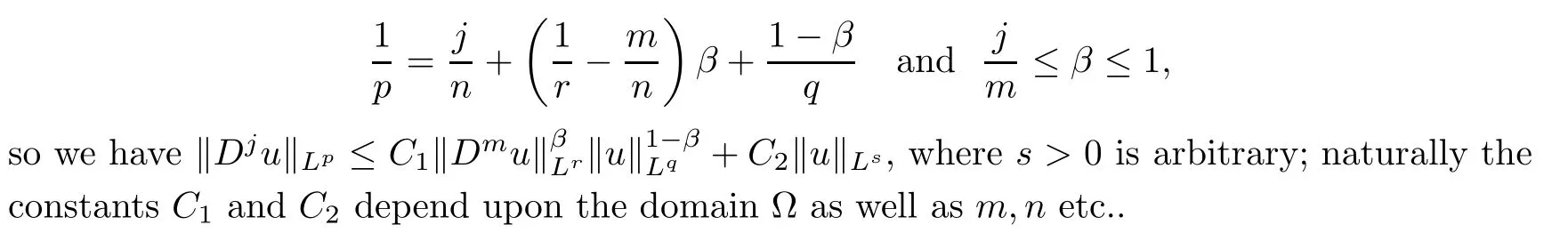
The following two lemmas are standard compactness results and will help us get the strong convergence of solutions:
Lemma 2.3([1,2])(Aubin-Lions Lemma) Let B0,B and B1be three Banach spaces with B0⊆B⊆B1.Suppose that B0is compactly embedded in B and that B is continuously embedded in B1.For 1≤p,q≤+∞,let

Then,
(i)if p<+∞,then the embedding of W into Lp([0,T];B)is compact;
(ii)if p=+∞and q>1,then the embedding of W into C([0,T];B)is compact.
Lemma 2.4([4])(Egoroffs theorem about uniform convergence) Let fn→f a.e.in Ω,with a bounded measurable set in Rn,with f finite a.e.Then,for any∊>0,there exists a measurable subset Ω∊⊂Ω such that|ΩΩε|<∊and fn→f uniformly in Ω∊.Moreover,if

we have fn→f strong in Ls,for any s∈[1,p).
ProofSince fn→f a.e.in Ω and fnis uniformly bounded in Lp(Ω),due to Egoroff’s theorem,we have

3 Faedo-Galerkin Approximation
In this section,we construct the approximate system to the original problem by using the Faedo-Galerkin method.We proceed similarly in[5]and[6].
3.1 Approximate system
In order to prove the global existence of weak solutions to the α-model regularization for the three-dimensional Euler-Poisson equations,we consider the following approximate system:

The extra terms−η∇ρ−6and−δρ∇Δ3ρ are necessary to keep the density bounded and bounded away from below with a positive constant for all time.This enables us to takeas a test function to derive the B-D entropy.The term r0u is used to control the density near the vacuum.−α2Δutis used to make sure that√ρu is a strong convergence in L∞([0,T];L2)at the last approximate level.
Letting T>0,we define a finite-dimensional space Xn=span{φ1,···,φn},n∈N,where{φk}is an orthonormal basis of L2(T3)which is also an orthogonal basis of H1(T3).Let(ρ0,u0)∈C∞(T3)be some initial data satisfying ρ0≥ξ>0 for x∈T3for some ξ>0,and let the velocity u∈C([0,T];Xn)satisfy

Since Xnis a finite-dimensional space,all the norms are equivalence on Xn.Thus,u is bounded in C([0,T];Ck(T3))for any k∈N,and there exists a constant C>0 depending on k such that

Then the approximate of continuity equation is defined as follows:
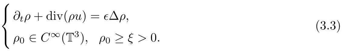
First,to show the well-posedness of the parabolic problem(3.3),we introduce the following lemma:
Lemma 3.1([8]) Let T3be a domain of class C2,θ,θ∈(0,1),and let u∈C([0,T];Xn)be a given vector field.If the initial data ρ0≥ζ>0,ρ0∈C2(T3),then problem(3.3)possesses a unique classical solution ρ=ρu.More specifically,

Furthermore,because u∈C([0,T];Xn)is a given vector field,by using the bootstrap method and Lemma 3.1,it is easy to prove that system(3.3)exists a unique classical solution ρ∈C1([0,T];C7(T3)).Moreover,if 0<ρ≤ρ≤ρ and divu∈L1([0,T];L∞(T3)),through the maximum principle it provides ρ(x,t)≥0.
Then if we define Lρ=∂tρ+div(ρu)−∊Δρ,by direct calculation we can obtain


Next we will show that the solution of equation(3.3)depends on the velocity u continuously.Let ρ1,ρ2be two solutions with the same initial data,that is,

Subtracting the above two equations,multiplying the resulting equation by−Δ(ρ1−ρ2)and integrating by parts with respect to x over T3,we have
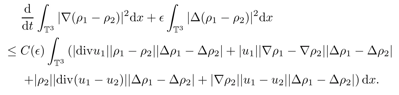
Since ρ1and ρ2satisfy Lemma 3.1,by using Cauchy-Schwartz inequality,Poincaré’s inequality and Gronwall’s inequality,we can obtain

Moreover,for u∈C([0,T];Xn)being a given vector field,by using the bootstrap method and compactness analysis,we can prove that

Thus if we introduce the operator S:C([0,T];Xn)→C([0,T];C7(T3))by S(u)=ρ,we have the following proposition:
Proposition 3.2If 0<ρ≤ρ≤ρ,ρ0∈C∞(T3),u∈C([0,T];Xn),then there exists an operator S:C([0,T];Xn)→C([0,T];C7(T3))satisfying that
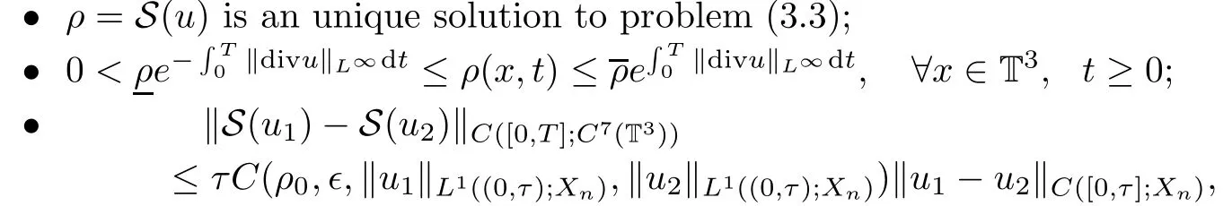
for any τ∈[0,T]and u1,u2∈MK={u∈C([0,T];Xn);‖u‖C([0,T];Xn)≤k,t∈[0,T]}.
Remark 3.3Proposition 3.2 suggests that the operator S is Lipschitz continuous for sufficiently small time t.
3.2 Fadeo-Galerkin approximation
Next,we hope to solve the momentum equation on the space Xnby using the Faedo-Galerkin approximation method.To this end,for given ρ=S(u),we are looking for an approximate solution un=C([0,T];Xn)satisfying


for any test function ϕ∈Xn.
To solve(3.7),we follow the same arguments as in[5,6,9],and introduce the following family of operators:

In a fashion similar to[9],it is easy to check that the operater M[ρ]satisfies the following operators:

for some α>0,and all ρ1,ρ2∈L1(T3),such that ρ1,ρ2≥ρ>0.
ProofHere we omit the proof;for more details,we refer readers to[5,6,9]. □
By using the operators M and ρ=S(un),the integral equation(3.7)can be rephrased as

In view of Lipschitz continuous estimates for S and M−1,equation(3.8)can be solved by the fixed-point theorem of Banach for a short time[0,T′],where T′≤T,on the space C([0,T];Xn).Thus there exists a unique local-in-time solution(ρn,un,Φ(ρn))to(3.3)and(3.8).Next we will extend this local solution that we have obtained to be a global one.
Differentiating(3.7)with respect to time t,taking φ=unand integrating by parts with respect to x over T3,we have the following energy estimate:

First,we estimate the terms on the left hand side one by one as follows:
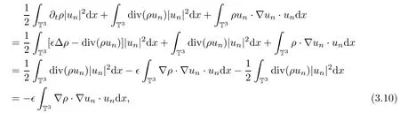
and where we use the approximate mass equation(3.3)and integration by parts:

Next we will deal with the cold pressure and high order derivative of the density terms as follows:
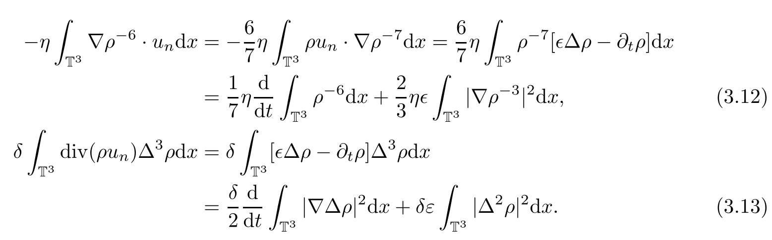
Finally,we will estimate the Poisson term on the right hand side as follows:

where we have used equation(1.3)3.
Then,substituting(3.10)–(3.14)into(3.7)and integrating the resulting equation with respect to t over[0,T]yields
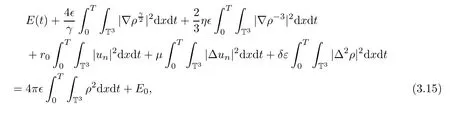
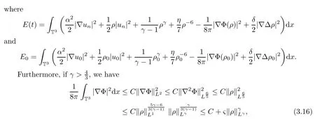
where 0<ς≪1 is a fixed constant,C is a generic positive constant independent of∊,η,δ,r0,and we have also used conservation of mass,Sobolev inequality,and Young’s inequality.
Then substituting(3.16)into(3.15)we get

where ς′is a sufficient small positive constant,and C is a generic positive constant depending only on the initial data and T.

Thus the energy inequality(3.20)yieldswhere C(∊,δ)denotes a positive constant depending particularly on∊,δ,but independent of n,and due to dimXn≤+∞and(3.5),the density is bounded and bounded away from below with a positive constant,which means that there exists a constant c>0 such that

for all t∈[0,T∗).Moreover,the energy inequality also gives us

which,together with(3.21),(3.22)and energy inequality,implies that

where we used the fact that all the norms are equivalent on Xn.Then we can repeat the above argument many times and,using the compactness analysis,we can obtain un∈C([0,T];Xn),so we can extend T∗to T.Thus there exists a global solution(ρn,un,Φ(ρn))to(3.3),(3.7)for any time T.
To conclude this part,we have the following proposition on the approximate solutions(ρn,un,Φ(ρn)):
Proposition 3.4Let(ρn,un,Φ(ρn))be the solutions of(3.3),(3.7)on(0,T)×T3constructed above.Then the solutions must satisfy the energy inequality(3.20).In particular,we have the following estimates:

3.3 Passing to the limits as n→∞.
We perform first the limit with n→∞,∊,η,δ,r0>0 being fixed.Based on the above estimates,which are uniform on n and in accordance with the Aubin-Lions Lemma,we have the following compactness results:
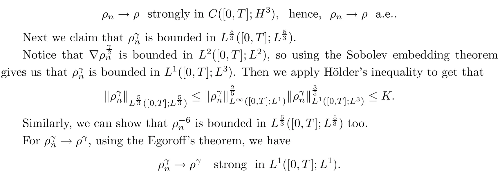
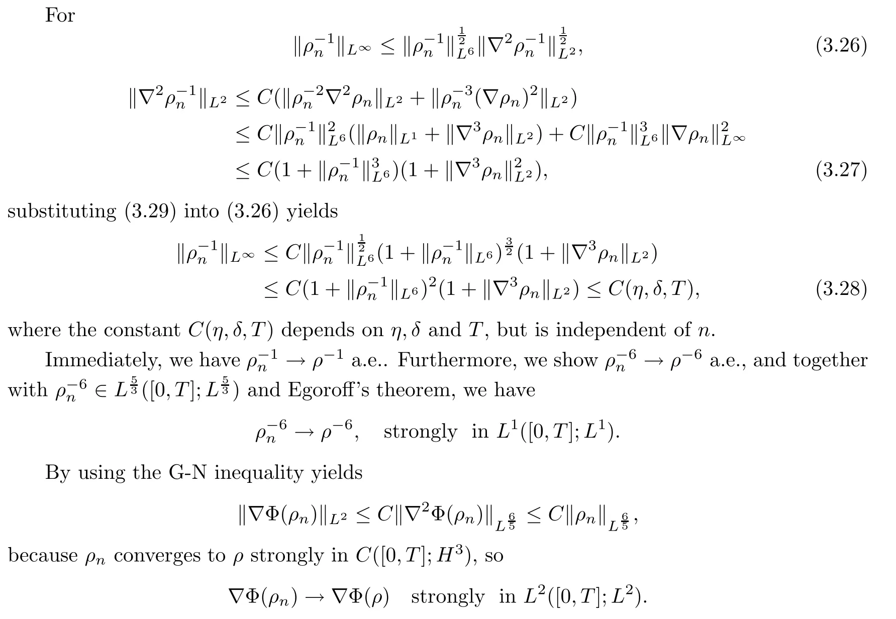
3.3.1Step 1Convergence of ρn,Pressure∇and gravitational force∇Φ(ρn)
Lemma 3.5The following estimates hold for any fixed positive constants∊,η,δ and r0:
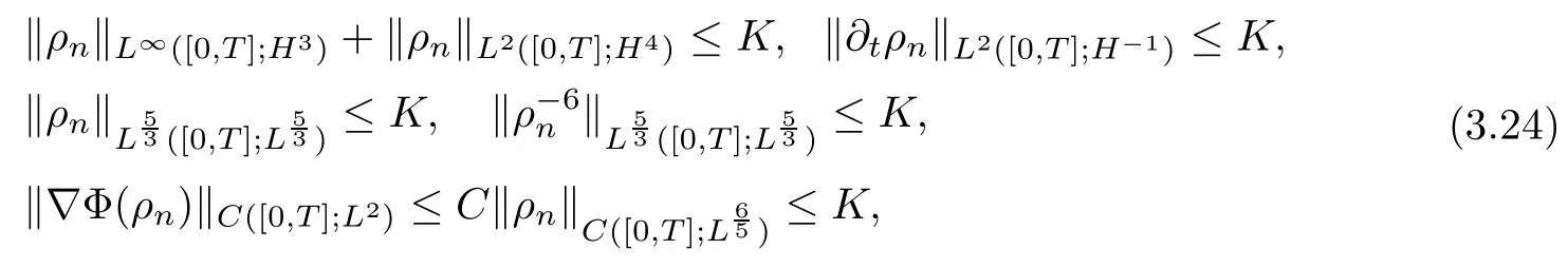
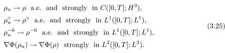
where K is independent of n,and depends on∊,η,δ,r0,initial data and T.Furthermore,up to an extracted subsequence,
ProofBy(3.3),we have that

holds for any ϕ∈L2([0,T];H1),which yields∂tρn∈L2([0,T];H−1).
This,together with ρn∈L∞([0,T];H3)TL2([0,T];H4),and using the Aubin-Lions Lemma,allows us to claim that ρn∈C([0,T];H3),so,up to a subsequence,we have
Next,we show that the density is bounded away from zero with a positive constant for all time t∈[0,T]by using the Sobolev inequality.
The proof of this lemma is complete. □
3.3.2Step 2Convergence of ρnun−α2Δun
Lemma 3.6Up to an extracted subsequence,

ProofFrom the energy estimates,we know that unis bounded in L∞([0,T];H1),so up to a subsequence,we have un⇀u in L∞([0,T];H1).
Recall that ρn→ρ strongly in C([0,T];H3),so we have

Moreover,since ρn∈L∞([0,T];H3),and un∈L∞([0,T];C∞),we can show that
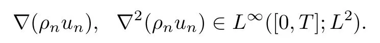
Together with ρnun∈L∞([0,T];L2),we have ρnun∈L∞([0,T];H2).Next,in order to use the Aubin-Lions Lemma,we only need to prove that

Since

based on the energy estimates,it is easy to check that∂t(ρnun−α2Δun)∈L2([0,T];H−3),so by using the Aubin-Lions Lemma,we can show

Thus the proof of this lemma is complete. □
3.3.3Step 3Convergence of nonlinear diffusion terms

Thus we have
With the above compactness results in hand,we are ready to pass to the limits as n→∞in the approximate system(3.3),(3.7).Thus,we can show that(ρ,u,Φ)solves
and for any test function ϕ,the following holds:

Thanks to the lower semicontinuity of norms,we can pass to the limits in the energy estimate(3.20),and we have the following energy inequality in the sense of distributions on(0,T):

Thus,we have the following proposition on the existence of weak solutions at this level approximate system:
Proposition 3.7There exists a weak solution to the following system:

with suitable initial data,for any T>0.In particular,the weak solutions(ρ,u,Φ)satisfy the energy inequality(3.32).
4 B-D Entropy and Passing to the Limits as∊,µ→0
In this section,we deduce the B-D entropy estimate for the approximate system in Proposition 3.7,which was first introduced by Bresch and Desjardins in[10];this B-D entropy will give a higher regularity of the density and will help us to get the compactness of ρ.By(3.24),(3.28)and u∈L2([0,T];H2),we have

4.1 B-D entropy

Substituting(4.3)–(4.5)into(4.2)and integrating it with respect to the time t over[0,T],we have


where we have used the energy inequality(3.32).Then we need to control the rest of the terms on the right hand side of(4.6):
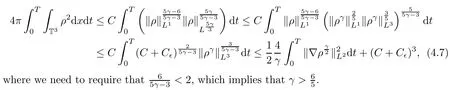
Next,we control the terms I4−I11as follows:

For some large fixed constant s>0,

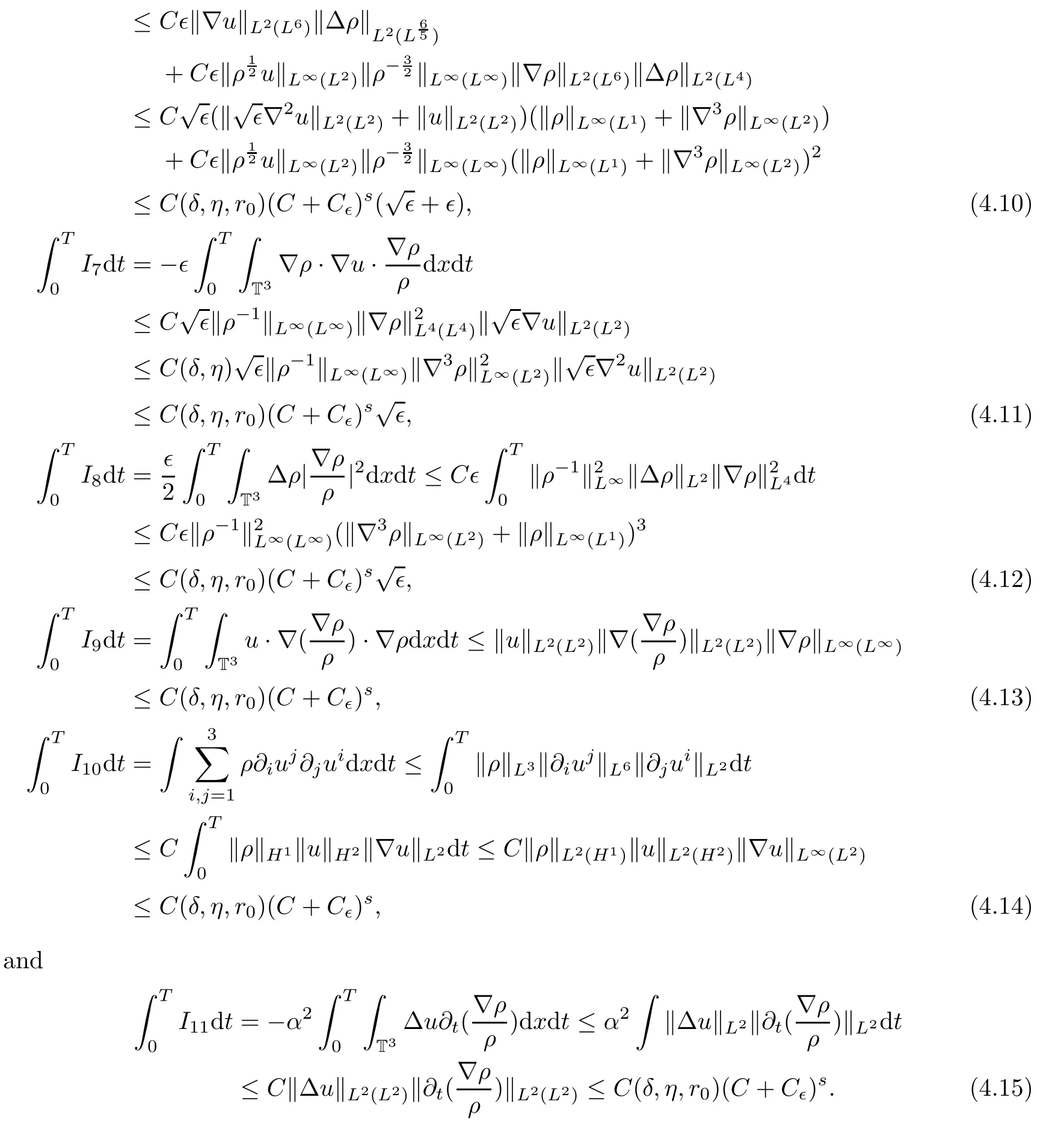
Then,substituting(4.7)–(4.15)into(4.2),we have

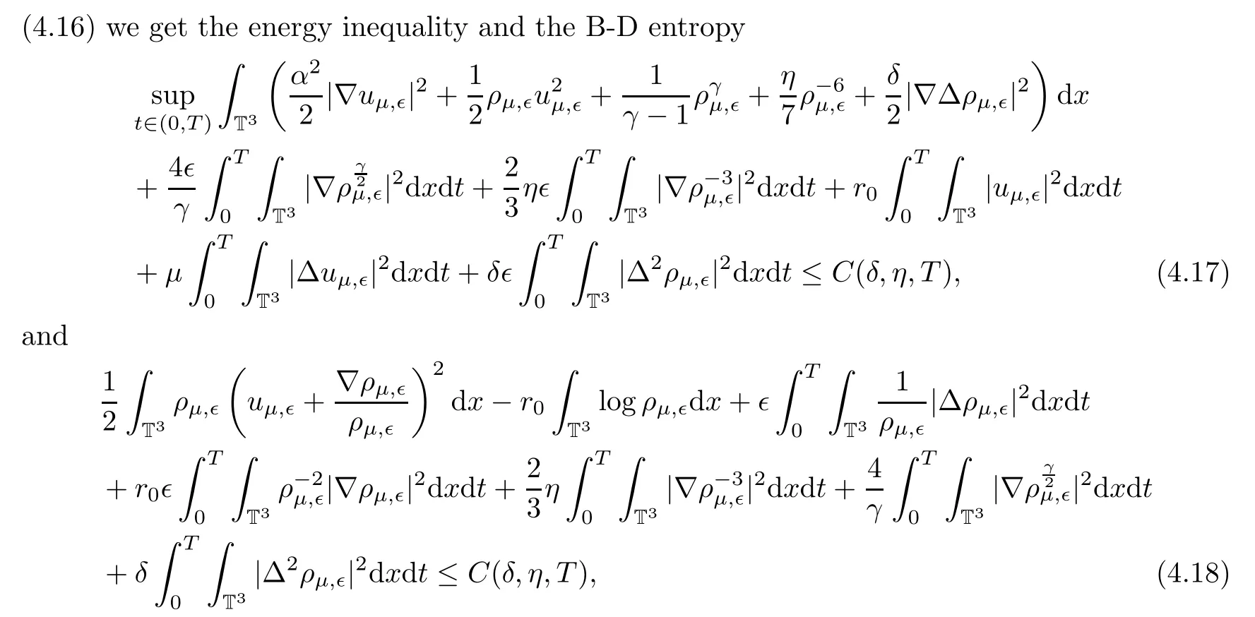
where C(δ,η,T)denotes that C particularly depends on δ,η and time T.
4.2 Passing to the limits asµ,∊→0
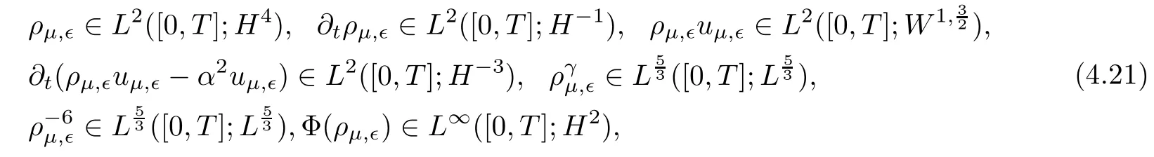
We use(ρµ,∊,uµ,∊,Φ(ρµ,∊))to denote the solutions at this level of approximation.From(4.17)and(4.18),it is easy to show that(ρµ,∊,uµ,∊,Φ(ρµ,∊))has the following uniform regularities:

Lemma 4.2Letting(ρµ,∊,uµ,∊,Φ(ρµ,∊))be weak solutions to(3.33),in combination with(4.19)and(4.20),we have
and using the Aubin-Lions Lemma,we have the following compactness results:

ProofThe proof is similar to the compactness analysis in Section 3,so for simplicity,we omit the details here. □
With the above compactness results in hand,we pass to the limits asµ=∊→0.Here we only focus on the terms involving∊andµ.First,because ρµ,∊is bounded in L∞(H3)TL2(H4)uniformly on∊,we have that
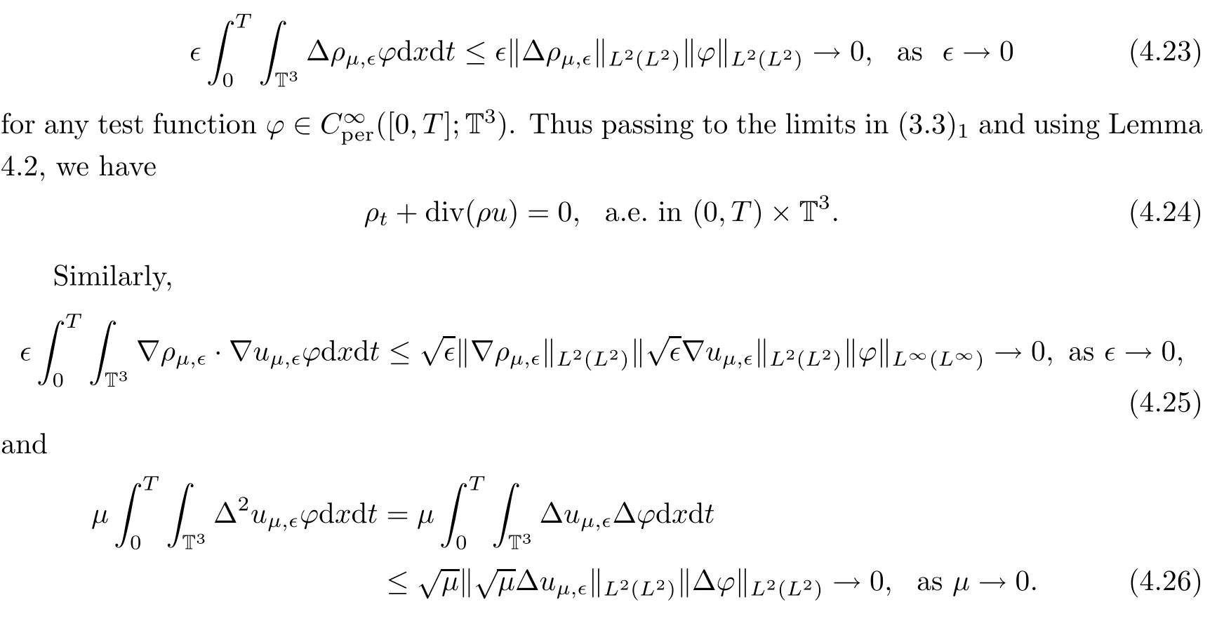
So passing to the limits asµ=∊→0 in(3.33),we have that

holds in the sense of distribution on(0,T)×T3,and that

Furthermore,thanks to the lower semi-continuity of the convex function and the strong convergence of ρµ,∊,uµ,∊,Φ(ρµ,∊),we can pass to the limits in the energy inequality(3.32)and B-D entropy(4.17)asµ=∊→0 with δ,η,r0being fixed as follows:
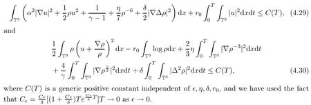
Thus,to conclude this part,we have the following proposition:
Proposition 4.3There exist the weak solutions to systems(4.24),(4.26)and(4.27)with suitable initial data,for any T>0.In particular,the weak solutions(ρ,u,Φ)satisfy the energy inequality(4.29)and the B-D entropy(4.30).
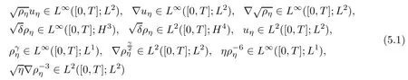
5 Passing to the Limits as η→0
In this section,we pass to the limits as η→0 with δ,r0being fixed.We denote that(ρη,uη,Φ(ρη))are weak solutions at this level.From Proposition 4.3,we have the following regularities:
It is easy to check that we have the same estimates as in Lemma 4.2 in terms of the level with η,thus we deduce the same compactness for(ρη,uη,Φ(ρη))as follows:

Thus,at this level of approximation,we only focus on the convergence of the term η∇.
Here we state the following lemma:
Lemma 5.1For ρηdefined as in Proposition 4.3,we have that
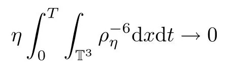
as η→0.
ProofThe proof is inspired by Vasseur and Yu[12].From the B-D entropy(4.30),we have that
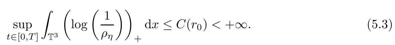
Note that

is a convex continuous function.Moreover,in combination with the property of the convex function and Fatou’s Lemma,this yields
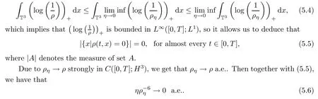
Moreover,using the interpolation inequality,that yields

This,together with(5.6)and Eogroff’s theorem,yields

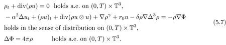
Thus,by using the compactness results(5.2),we can pass to the limit as η→0 in(4.24),(4.27)and(4.28):
Similarly,due to the lower semi-continuity of convex functions,we can obtain the energy inequality and B-D entropy by passing to the limits in(4.29)and(4.30)as η→0,so we have

Thus,we have the following Proposition on the existence of weak solutions at this level of approximation:
Proposition 5.2There exist weak solutions to system(5.7)with suitable initial data,for any T>0.In particular,the weak solutions(ρ,u,Φ(ρ))satisfy the energy inequality(5.8)and the B-D entropy(5.9).
6 Passing to the Limits as δ,r0→0
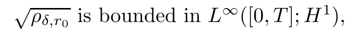
At this level,the weak solutions satisfy the energy inequality(5.8)and the B-D entropy(5.9),thus we have the following regularities:

Next,we will proceed to examine the compactness arguments in several steps.
6.1 Step 1 Convergence of
Lemma 6.1Letting(ρδ,r0,uδ,r0Φ(ρδ,r0))satisfy Proposition 5.2,we have

As a consequence,up to a subsequence,converges almost everywhere and strongly in L2([0,T];L2),which means that

Moreover,we have
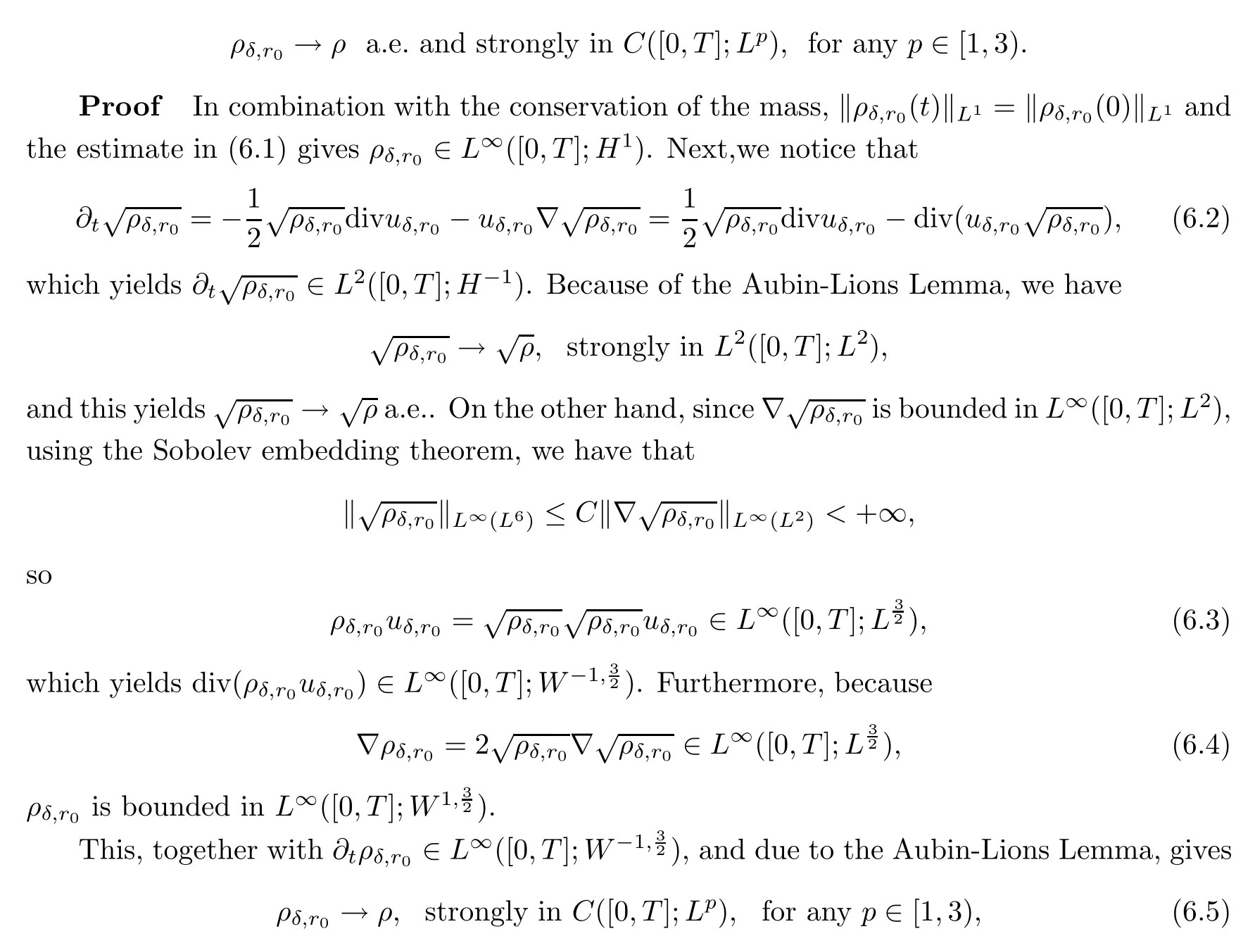
and hence,we have

Thus the proof of Lemma 6.1 is complete. □
6.2 Step 2 Convergence of
Lemma 6.2The termsatisfies the regularityand up to a subsequence,we havea.e.,andstrongly in L1([0,T];L1).
ProofThe proof is as the same as it is in Section 2,so we omit the details here. □
6.3 Step 3 Convergence of the momentum and the term−α2Δ
Lemma 6.3Up to a subsequence,the momentum and α-regular ofis

Note that we can define u(x,t)=m(x,t)/ρ(x,t)outside the vacuum set{x|ρ(x,t)=0}.
ProofSince

In order to apply the Aubin-Lions Lemma,we also need to show that

Actually,using the momentum equation(5.7)2,it is easy to check that

Hence,using the Aubin-Lions Lemma,Lemma 6.3 is proved. □
6.4 Step 4 Convergence of
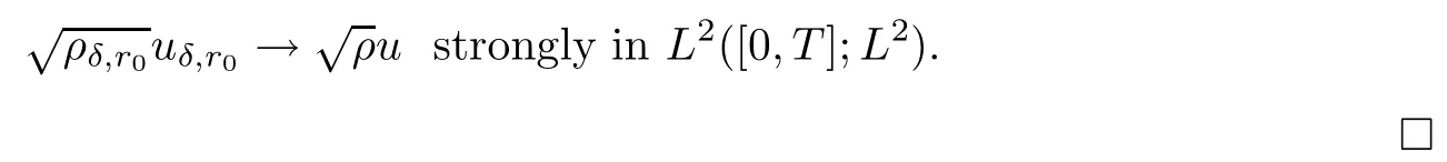
Lemma 6.4We havestrongly in L2([0,T];L2),and there exists a function u(x,t)such that m(x,t)=ρ(x,t)u(x,t)and
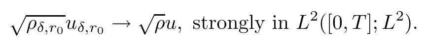
ProofRecalling Lemma 6.3,we define velocity u(x,t)by setting u(x,t)=m(x,t)/ρ(x,t),so we have m(x,t)=ρ(x,t)u(x,t).
Moreover,Fatou’s lemma yields that


as r0=δ→0 and M→+∞.Thus we have proven that
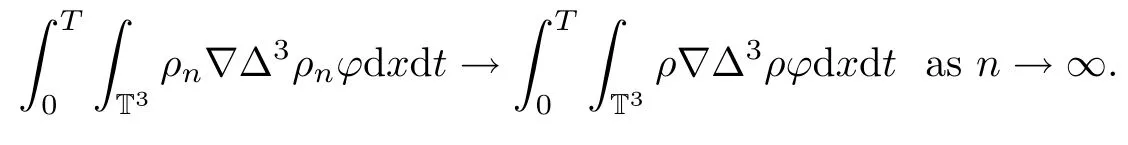
6.5 Step 5 Convergence of the terms

Focussing on the most difficult term,

Similarly,we can deal with the other terms from

With all of the above compactness results,we can pass to the limits in(5.7)as δ→0,so we have that

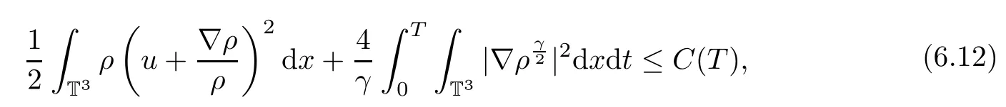
Furthermore,thanks to the lower semi-continuity of the convex function,we can obtain the following energy inequality and B-D entropy by using the limits as δ=r0→0:

and
Thus we have completed the proof of Theorem 1.2.
猜你喜欢
科普童话·神秘大侦探(2021年12期)2021-01-19
电脑知识与技术·经验技巧(2017年9期)2018-02-24
中国摄影(2017年11期)2017-11-22
创作(2017年5期)2017-11-13
三联生活周刊(2016年43期)2016-10-28
小学生·多元智能大王(2016年6期)2016-05-14
家教世界·创新阅读(2014年11期)2014-12-15
小说评论(2013年1期)2013-11-15
世纪(2012年1期)2012-07-23
恋爱婚姻家庭(2009年6期)2009-06-04
 Acta Mathematica Scientia(English Series)2021年3期
- Acta Mathematica Scientia(English Series)的其它文章
- SEQUENCES OF POWERS OF TOEPLITZ OPERATORS ON THE BERGMAN SPACE∗
- A REMARK ON GENERAL COMPLEX(α,β)METRICS∗
- MULTIPLE SOLUTIONS FOR THE SCHRDINGER-POISSON EQUATION WITH A GENERAL NONLINEARITY∗
- HOMOCLINIC SOLUTIONS OF NONLINEAR LAPLACIAN DIFFERENCE EQUATIONS WITHOUT AMBROSETTI-RABINOWITZ CONDITION∗
- SHARP BOUNDS FOR TOADER-TYPE MEANS IN TERMS OF TWO-PARAMETER MEANS∗
- THE PROXIMAL RELATION,REGIONALLY PROXIMAL RELATION AND BANACH PROXIMAL RELATION FOR AMENABLE GROUP ACTIONS∗