Evaluation of second-order Zeeman frequency shift in NTSC-F2*

Jun-Ru Shi(施俊如) Xin-Liang Wang(王心亮) Yang Bai(白杨) Fan Yang(杨帆)Yong Guan(管勇) Dan-Dan Liu(刘丹丹) Jun Ruan(阮军) and Shou-Gang Zhang(张首刚)

1National Time Service Center,Chinese Academy of Sciences,Xi’an 710600,China

2Key Laboratory of Time and Frequency Primary Standards,Chinese Academy of Sciences,Xi’an 710600,China

3University of Chinese Academy of Sciences,Beijing 100049,China

Keywords: caesium atomic fountain clock,second-order Zeeman frequency shift,C-field,magnetic shielding

1. Introduction

Caesium atomic fountain clock is a primary frequency standard device which realizes the SI“second”.[1]Several laboratories worldwide are studying atomic fountain clock to improve its performance, which includes the two extremely important parameters,that is,frequency accuracy and frequency stability.[2-8]

Recently,a new caesium atomic fountain clock NTSC-F2 has just been developed and put into operation at the National Time Service Center (NTSC). To evaluate the frequency uncertainty, it must be corrected for the following several frequency shifts: second-order Zeeman frequency shift,[9]collisional frequency shift,[10]gravitational red frequency shift,[11]black-body radiation frequency shift,[12]and so on. Among these frequency shifts, the second-order Zeeman frequency shift is the dominant frequency correction and its uncertainty largely limits the improvement of frequency accuracy. It is induced by C-field, which is generated deliberately over the atomic flight region to remove the degeneracy of the magnetic sub-states.

Over the years second-order Zeeman frequency shift has been studied widely with great improvements.[13-16]Several techniques are used to measure the C-field precisely and evaluate this frequency shift,such as magnetically sensitive Ramsey transition,[17]stimulated Raman transition,[18]and slow frequency transition.[19]In order to identify the central fringe of the magnetically sensitive Ramsey pattern, we can compare the measured magnetically sensitive Ramsey pattern with the theoretically predicted one,which is obtained by integrating the measured C-field along the atomic flight trajectory.[14]Another method to identify the central fringe is to measure the central fringe step by step with the atomic launching height increasing.[20]To evaluate the second-order Zeeman frequency shift uncertainty induced by the fluctuation of the Cfield,the interrogating microwave frequency is locked on this central fringe and this central frequency fluctuation is recorded in time domain. At present, the worldwide state-of-theart caesium atomic fountain clocks including PTB-CsF2,[21]NIST-F2,[22]FO2 double fountains at LNE-SYRTE,[23]NPLCsF3,[24]MTsR-F2 at VNIIFTRI[6]have realized the evaluation of second-order Zeeman frequency shift with the uncertainty up to the order of 10-17. This is of great importance to improve the performance of caesium atomic fountain clock.

The uncertainty of second-order Zeeman frequency shift is dominated by C-field instability and nonuniformity. In this paper, by applying a high-precision current supply to C-field solenoid and high-performance magnetic shieldings,we realize a significant improvement of second-order Zeeman frequency shift uncertainty compared with our first caesium atomic fountain clock NTSC-F1. At the same time, by designing a doubly wound C-field solenoid instead of a singly wound one as in NTSC-F1, we achieve a more uniform Cfield. On the basis of the improved C-field,the first evaluation of second-order Zeeman frequency shift of NTSC-F2 has been performed and is described in the following sections. In traditional magnetically sensitive Ramsey transition method,we construct the C-field profile and obtain the central frequency of the magnetically sensitive Ramsey transition fringe. Meanwhile,by monitoring the variation of this central frequency for ten consecutive days,we obtain the range less than±0.45 Hz.Lastly, we realize the improvement of second-order Zeeman frequency shift and obtain this fractional frequency shift of 131.03×10-15with the uncertainty of 0.10×10-15.

2. Theoretical study of second-order Zeeman frequency shift

In C-fieldBin units of T, the frequencies of caesium ground-state hyperfine transition(ΔF=1, ΔmF=0)in units of Hz are given by the Breit-Rabi formula, which are shown(approximate to second order)as follows:[25]

wheremFis the projection of the angular momentum operatorFalong the C-fieldB,namely magnetic quantum number;νhfs= 9192631770 Hz is the unperturbed caesium groundstate hyperfine transition frequency betweenF=3 andF=4;x=(gJ-gI)μBB/(hνhfs);gJandgIare the electronic and nucleargfactors;μBis Bohr’s magneton;andhis Planck’s constant.

According to Eq. (1), we obtain the frequencies of the transitions|F= 3,mF= 0〉 →|F= 4,mF= 0〉and|F=3,mF=-1〉→|F=4,mF=-1〉as

Above all, as long as we find the central fringe of the magnetically sensitive Ramsey transition|F=3,mF=-1〉→|F=4,mF=-1〉experimentally, the evaluation of secondorder Zeeman frequency shift is realized.

3. C-field profile construction

During the evaluation of second-order Zeeman frequency shift,the mentioned central frequency of the magnetically sensitive Ramsey transitionF=3,mF=-1〉→|F=4,mF=-1〉is determined by the time integral of the C-field along the atomic flight trajectory:[26]

whereTis the atomic flight time above Ramsey cavity,B(t)is the C-field atoms experience at timet. In the above approximation,Tis divided intoNparts,Biis the C-field of thei-th part andtiis the corresponding time. Thus,we could use the magnetically sensitive Ramsey transition to measure the C-field by measuring the frequency of the central fringe at a series of discrete positions,as shown in Fig.1.

Fig.1. The deconvolution model for constructing C-field profile in the Ramsey method.

Assuming the reference point is right at the top of Ramsey cavity with the heighth=0 cm,and the C-field below the reference point isB0,Zeeman frequency isνz(h)correspondingly. According to Eq.(5)we could calculateB0as

where the coefficientc=(1/7.0083)nT/Hz.

As shown in Fig. 1, we suppose the C-field of the 1st,2nd,...,n-th points above the reference point areB1,B2,...,Bn,the corresponding heights areh1,h2,...,hn,and the corresponding Zeeman frequencies areνz(h1),νz(h2),...,νz(hn).The time atoms spend passing from the apogee at each launching height to positions beneath the 1st,2nd,...,n-th points areT1,T2,...,Tn,respectively. Therefore,by a deconvolution of the time-averaged C-field and the atoms’ flight time,[27]we can obtain the C-field of the 1st, 2nd, ...,n-th points above the reference point as follows:

In this Ramsey method, we could map the C-field precisely using the atoms as a probe.

4. C-field design

According to the theoretical calculation in Section 2,we could evaluate the second-order Zeeman frequency shift by measuring the magnetically sensitive frequencyν-1instead ofν0. Here,ν-1is 106times as sensitive to the fluctuation of Cfield asν0. However,because of the C-field’s nonuniformity,the central fringe of the magnetically sensitive Ramsey transition|F=3,mF=-1〉→|F=4,mF=-1〉will deviate from the Rabi pedestal, it is difficult to identify the central fringe from the large amounts of Ramsey fringes to measure the frequencyν-1. Above all,it is of great importance to produce a uniform and stable C-field.

C-field is composed of three parts, those are, solenoid’s magnetic field, magnetic shieldings’ residual magnetic field and the Earth’s magnetic field (about 105nT). In the NTSCF2 magnetic field system, four cylindrical magnetic shieldings made of JIS C 2531 soft metal (thickness: 2 mm, high magnetic permeability: 1.8×105) are assembled around the solenoid to provide a uniform C-field deliberately over the atomic flight region, they are coaxial with Ramsey cavity.Each magnetic shielding is closed with upper and lower endcaps,and each has a 50 mm diameter hole in the center for the vacuum system. We also place compensation coils at the bottom of magnetic shieldings to guarantee the axial C-field far away from zero,which might induce Majorana transitions[28]In order to increase the selection efficiency, a compensation coil is applied in the lower selection zone to minimize the background magnetic field gradient. Figure 2(a)illustrates the structure of NTSC-F2 magnetic system.

In order to measure the central axial shielding factor of the assembled magnetic shieldings,[29-31]we wind a horizontal coil around the magnetic shieldings symmetrically. By measuring the central axial magnetic field strength with a fluxgate magnetometer, we obtain the distributions of the axial magnetic field component in different magnetic fields:Bb+,Bb,Ba+,Ba-. The subscripts b and a indicate the measurements are implemented before and after the magnetic shieldings being assembled respectively,+and-indicate the external coil’s current in two different directions. Therefore,applying the shielding factor expression

we obtain the total central axial shielding factor along the atomic flight trajectory as shown in Fig. 2(b). We can obviously see that the shielding factor in the middle part is at the maximum level of 3×105. Due to the holes at both ends of the magnetic shieldings, the shielding factor gradually attenuates from the middle to its both ends. Compared with the traditional method by measuring the background magnetic field strength straightforwardly,[32]this method has eliminated the measurement error induced by the residual magnetic field of the magnetic shieldings, and is applicable to measure the high-performance magnetic shieldings. At the same time,we use a high-precision current supply (brand: Keithley, model:2614B)for C-field solenoid to achieve a stable C-field.

Fig.2.Schematic diagrams of NTSC-F2 magnetic system:(a)four concentric cylindrical magnetic shieldings with endcaps, C-field solenoid is placed inside the innermost magnetic shielding, two compensation coils are set at the bottom of magnetic shieldings and in the lower selection zone respectively. (b)Central axial magnetic shielding factor along atomic flight trajectory.

Traditionally, the C-field solenoid is spirally wound by a single wire from the top to the end as the one installed in NTSC-F1. If the two ends of this wire outgo from each nearby end-caps separately for power in and out,then the hole punched at the bottom end-caps would reduce the C-field uniformity of the crucial atomic flight region (in the lower part)seriously. Thus, we usually lead the bottom end of this wire upward straightly and combine with the top end of this wire,outgoing together from the top end-caps. However,according to the Biot-Savart law with the C-field solenoid parameters,the bottom end of this wire along C-field solenoid sidewall would generate a radial magnetic field on the central axis at about 0.3 nT,which affects the C-field uniformity and orientation to a certain extent,inducing the Ramsey frequency pulling shift.[33]Concerning this issue, we propose a doubly wound C-field solenoid design as shown in Fig. 3, where the double wires are red and black nonmagnetic enameled copper wires separately. Here the double wires spirally wind around the teflon tube from top to bottom, then separate into two single wires and symmetrically go along the sidewall straight up to the top separately. On the top,the two wires combine together again for current in. So the radial magnetic fields generated by two single wires on the central axis cancel each other out to implement a more uniform C-field. It has a total of 97 turns and an input current 1.007 mA. The size parameters of magnetic shieldings and C-field solenoid are listed in Table 1.

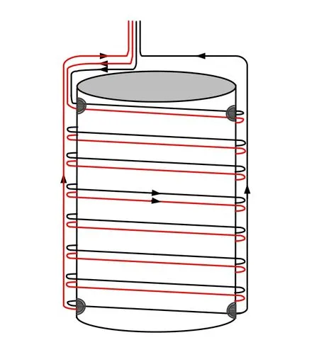
Fig.3. Doubly wound C-field solenoid.

Table 1. Size parameters for NTSC-F2 magnetic shieldings and C-field solenoid(in millimeters). The four cylindrical magnetic shieldings are numbered as 1,2,3,4 from the innermost to outermost sequentially.

5. The evaluation of second-order Zeeman frequency shift

The physical and optical system of NTSC-F2 has been described in Ref. [34] in detail. After launching, the atoms distributed in the 9 sub-levels of stateF=4 fly through Ramsey cavity twice without selection.By scanning the interrogating microwave frequency in step 0.2 Hz(with the microwave field amplitude corresponding to aπ/2 pulse area)and recording the atoms’population in stateF=3 andF=4 respectively,we obtain 7 obvious Ramsey patterns corresponding toσtransitions(ΔmF=0)shown in Fig.4.Because the Ramsey cavity resonant frequency deviates fromνhfs,these transition patterns are not medianly zygomorphic. Meanwhile, the tiny signals corresponding toπtransitions(ΔmF=±1)induced by radial magnetic field are less than 1.7%, we deduce that the C-field is well aligned with the clock central axis.

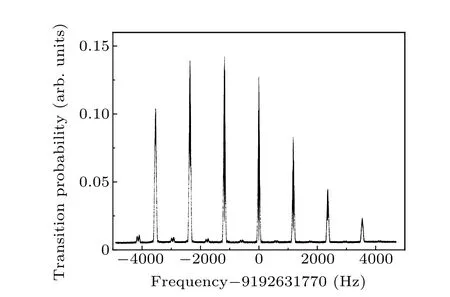
Fig. 4. Microwave spectrum in Ramsey cavity (π/2 pulse area) without selection: 7 Ramsey patterns,from left to right corresponding to σ transitions mF =-3,-2,...,3,respectively.

Because the atoms in states|F=4,mF/=-1〉do not contribute to this magnetically sensitive Ramsey transition signal,it is necessary to perform a state selection process to improve frequency accuracy and stability. By the application of compensation coil in selection zone as mentioned in Section 4,the magnetic field gradient is reduced from the order of 103nT/cm to 102nT/cm, which eases the selection of atoms in state|F=3,mF=-1〉. Based on the optimized magnetic field in the selection zone,we scan the selecting microwave frequency and obtain the selecting microwave frequency between states|F=4,mF=-1〉and|F=3,mF=-1〉as 9192435142 Hz.By setting the selecting microwave frequency to this value,we realize the selection of atoms in state|F=3,mF=-1〉.

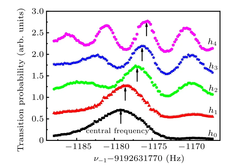
Fig. 5. The magnetically sensitive Ramsey transition |F = 3,mF =-1〉→|F =4,mF =-1〉fringes of the first five launching heights and the corresponding heights are marked on the right. The arrow marks the central frequency at each height.

Substituting the structural parameters of NTSC-F2, we obtain the detuning frequency as Δν0=2.30 MHz when the atoms’ launching height ish0= 0 cm above the reference point. By slowly increasing the detuning frequency Δνifrom 2.30 MHz to 2.86 MHz with 0.02 MHz increment (correspondingn=28), we observe the number of Ramsey fringes increase and record the movement of central Ramsey fringe.When the launching height is low, the central frequency differences between the central Ramsey fringe and its adjacent Ramsey fringes are much larger (about 10 Hz) than the central Ramsey fringe frequency increment, so it is easy to distinguish which Ramsey fringe is central. Figure 5 shows the magnetically sensitive Ramsey transition|F= 3,mF=-1〉→|F=4,mF=-1〉fringes of the first five launching heights (h0,h1,h2,h3andh4), and each central frequency at the corresponding launching height is marked with an arrow. In these five signals, the square marked curve corresponds to the launching height ash0= 0 cm. Because of the nonuniformity of the microwave magnetic field of TE011mode in Ramsey cavity, there is an obvious Ramsey fringe with a tiny transition signal on its right side. This obvious fringe is exactly the central Ramsey fringe with the central frequency asν-1(h0)=9192630591.0 Hz and Zeeman frequency asνz(h0)=νhfs-ν-1(h0)=1179.0 Hz. The triangular marked curve corresponds to the detuning frequency as Δν1= 2.32 MHz, by comparing the Ramsey fringes of the first two heights, we find the central Ramsey fringe moving towards the right and the central frequencyν-1(h1)increasing by 0.6 Hz,i.e.,ν-1(h1)=9192630591.6 Hz. Meanwhile,the tiny transition signal becomes stronger. The dot-marked curve corresponds to the detuning frequency as Δν2=2.34 MHz.The number of Ramsey fringes increases to three and the central frequencyν-1(h2)increases to 9192630593.0 Hz. In the same method, we also find the central Ramsey fringes of the next two launching heights.

Above all, we obtain the relation between launching heighthiand detuning frequency Δνias follows:

where the local gravitational acceleration isg=9.79666 m/s2.[35]

Increasing the launching height up to the point 32 cm above the reference point and repeating the above measurement, we obtain the central Ramsey fringes and Zeeman frequencyνz(h)of the magnetically sensitive Ramsey transition|F=3,mF=-1〉→|F=4,mF=-1〉as a function ofh,as the dot-marked curve shown in Fig. 6. At the same time,we record the central frequencies of the two adjacent fringes,and obtain the variation of the two corresponding Zeeman frequencies as the square and triangle marked curves shown in Fig. 6. It obviously confirms that the frequency differences among these three curves are much larger than Zeeman frequency shift,which eases the identification of the central Ramsey fringe. With the increase of launching height, the two adjacent fringes gradually move towards the central Ramsey fringe.

Fig.6.NTSC-F2 three central Zeeman frequency variations of the magnetically sensitive Ramsey transition|F=3,mF =-1〉→|F=4,mF =-1〉with the launching height increasing.

From Fig. 6, we typically measure the central frequency asν-1(32 cm)=9192630593.6 Hz and Zeeman frequency asνz(32 cm)=1176.4 Hz during NTSC-F2 normal operation.Figure 7 shows the corresponding complete magnetically sensitive Ramsey transition|F=3,mF=-1〉→|F=4,mF=-1〉fringes and the arrow marks the central frequency.

With the C-field slowly drifting, the central fringe of the magnetically sensitive Ramsey transition may lose identity.After the above measurement,ν-1(32 cm)is immediately input to the control system as the initial estimate to identify and lock on this central fringe. Thus we have a good record of the central frequencyν-1fluctuation every four seconds over a ten-day-interval during NTSC-F2 normal operation continuously and obtain the result shown in Fig.8,in which the black dots indicate the average of central frequencies in every interval and error bars mean the variation ranges of central frequency.

Fig. 7. NTSC-F2 |F = 3,mF = -1〉 →|F = 4,mF = -1〉 Ramsey fringes during normal operation.

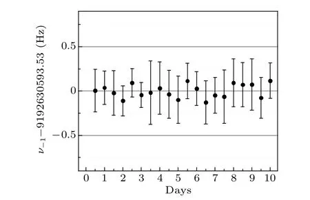
Fig.8. Temporal variation of central frequency ν-1 (32 cm)in NTSC-F2.

Combining Eq.(4)and noting that the Zeeman frequency mean value isνz=1176.47 Hz with the temporal variation range ofδνz(32 cm) =±0.45 Hz, we obtain the relative second-order Zeeman frequency shift during NTSC-F2 normal operation as

with the uncertainty arising from the instability and nonuniformity of C-field as[36]

In the evaluation of second-order Zeeman frequency shift we use an approximation〈B2〉=〈B〉2. Considering the Cfield nonuniformity along the atomic flight trajectory,〈B2〉=〈B〉2+σ2and the C-field standard deviation isσ, which describes the nonuniformity of C-field. After performing a correction to Eq.(4),the relative uncertainty of second-order Zeeman frequency shift arising from calculation approximation is expressed as[15]

In order to evaluate this contribution,we need to measure the C-field along the atomic flight trajectory. As mentioned in Section 3,the central Ramsey fringe in Fig.6 gives the information of time-integrated C-field.By deconvoluting,we could construct the actual C-field profile. When the atoms launching height ishi,the timeTj(j=1,2,...,i)atoms spend from the apogee to its lower nextj-th point as shown in Fig.1 could be expressed as

Substituting Eq. (14) and the above measured Zeeman frequencyνz(hi)into Eq.(8),we obtain the time-averaged Cfield along the atomic flight trajectory as shown in Fig.9. We can clearly see a bump near the Ramsey cavity, which may be attributed to two reasons: the effect of Ramsey cavity’s vacuum feedthroughs with high permeability and the effect of magnetic field leakage from the magnetic shieldings’end-caps holes. The data tells us that the C-field variation range is less than 0.5 nT within 30 cm. When the atoms are launched to the maximum height, 32 cm above the reference point, the standard deviation of the C-fieldσis 0.15 nT, less than 0.1% of the C-field mean value〈B〉= 167.85 nT. As a result, from Eq.(13)the relative uncertainty of second-order Zeeman frequency shift arising from calculation approximation is

Fig.9. The C-field profile of NTSC-F2.

The C-field fluctuation induces fluctuation of clock transitionF=3,mF=0→F=4,mF=0 frequency during NTSCF2 normal operation. The corresponding Allan deviation of clock transition frequency is shown in Fig. 10. These data tell us that the NTSC-F2 fractional frequency stability is better than 2.6×10-17.

Fig. 10. C-field instability induced total deviation of the frequency fluctuation on the clock transition F =3,mF =0 →F =4,mF =0 in NTSCF2. These data are obtained by measuring and translating the transition|F=3,mF =-1〉→|F=4,mF =-1〉frequency fluctuation into frequency shift on the clock transition.

Above all, the total relative uncertainty of second-order Zeeman frequency shift is 0.10×10-15. Comparing with NTSC-F1, the C-field nonuniformity and second-order Zeeman frequency shift uncertainty in NTSC-F2 are improved significantly[9]as listed in Table 2, which proves that this C-field design contribution to NTSC-F2 final performance is great.

Table 2. The improvement of C-field nonuniformity and secondorder Zeeman frequency shift uncertainty in NTSC-F2,compared with NTSC-F1.

Comparing the second-order Zeeman frequency shift uncertainty of NTSC-F2 with the worldwide state-of-the-art caesium atomic fountain clocks,which are on the order of 10-17,it is still too big to be neglected. According to Eq. (12), this gap is mainly attributed to the instability and magnitude of solenoid current, and consequently the C-field as well. Next,we plan to reduce the solenoid current and design a C-field dual servo system[13,22,37,38]to improve the C-field stability and to reduce the fractional uncertainty to the order of 10-17,which is realized by monitoring the C-field variation in slow frequency transition method and modulating the C-field solenoid’s input current in real time.

6. Conclusion

Second-order Zeeman frequency shift is a frequency bias induced by C-field, which limits the accuracy improvement of caesium atomic frequency standard. Concerning that NTSC-F1 C-field is not uniform and stable enough, we propose a doubly wound C-field solenoid. Also, by applying a high-precision current supply and high-performance magnetic shieldings, we obtain an improved C-field. Meanwhile,based on the improved magnetic field in selection zone, we perform a state selection process to obtain the atoms in magnetically sensitive state|F=3,mF=-1〉. Then we evaluate the second-order Zeeman frequency shift of NTSC-F2 for the first time in magnetically sensitive Ramsey transition method and construct a uniform C-field profile along the atomic flight trajectory. Subjected to the solenoid current instability, the second-order Zeeman frequency shift needs further improvement.Next we will reduce the solenoid current and design a Cfield dual servo system to improve the C-field stability,which could further reduce this uncertainty contribution to secondorder Zeeman frequency shift uncertainty and clock frequency stability.