Effects of magnetic field on electron power absorption in helicon fluid simulation

Mingyang WU (吴明阳), Chijie XIAO (肖池阶), Yue LIU (刘悦),

Xiaoyi YANG (杨肖易)1, Xiaogang WANG (王晓钢)1,3, Chang TAN (谭畅)4,5 and Qi SUN (孙琪)1,6

1 State Key Laboratory of Nuclear Physics and Technology, School of Physics, Fusion Simulation Center,Peking University, Beijing 100871, People’s Republic of China

2 Key Laboratory of Materials Modification by Laser, Ion and Electron Beams (Ministry of Education),School of Physics, Dalian University of Technology, Dalian 116024, People’s Republic of China

3 Harbin Institute of Technology, Harbin 150001, People’s Republic of China

4 Shaanxi Key Laboratory of Plasma Physics and Applied Technology,Xi’an 710100,People’s Republic of China

5 Xi’an Aerospace Propulsion Institute, Xi’an 710100, People’s Republic of China

6 School of Physics, Beijing Institute of Technology, Beijing 100081, People’s Republic of China

Abstract In this study, a code, named Peking University Helicon Discharge (PHD), which can simulate helicon discharge processes under both a background magnetic field greater than 500 G and a pressure less than 1 Pa, is developed.In the code, two fluid equations are used.The PHD simulations led to two important findings:(1)the temporal evolution of plasma density with the background magnetic field exhibits a second rapid increase(termed as the second density jump),similar to the transition of modes in helicon plasmas;(2)in the presence of a magnetic field,the peak positions of electron power absorption appeared near the central axis,unlike in the case of no magnetic field.These results may lead to an enhanced understanding of the discharge mechanism.

Keywords: helicon plasma, discharge process, numerical simulation

1.Introduction

Helicon plasmas exhibit desirable properties such as high plasma density, low-pressure operation, steady-state discharge, high power coupling efficiency, and no requirement of electrodes in the plasma region.In addition to their use in plasma research as well as in applications such as the Variable Specific Impulse Magnetoplasma Rocket, the helicon plasma thruster and the helicon double layer thruster [1–7], they are also used in materials processing owing to their several advantages [1, 8].

A unified theory on the discharge mechanism of helicon plasmas has not yet been established [9].Helicon plasmas mainly exhibit two coupling modes, electromagnetic and electrostatic.Electromagnetic modes are weakly damped and called helicon waves, whereas electrostatic modes are strongly damped and called Trivelpiece-Gould (T-G) waves[10–12].Chen pointed out that the Landau damping mechanism played an important role in helicon discharges [13];this was also verified experimentally [14].Further experimental studies showed that the number of fast electrons was insufficient to provide the full ionization, which proved that Landau damping is not important [15, 16].Several simulations on power deposition,such as those based on ANTENA2 and HELIC,indicate that T-G waves are essential components in the ionization mechanism[11,17].Further,the presence of T-G waves was verified experimentally [18].Currently, it is widely accepted that the helicon waves and T-G waves may be the main contributors to the ionization [1].

Table 1.Some helicon apparatuses and their typical operating parameters.

Numerical simulation is an efficient way to study helicon plasmas.Particularly,all the physical quantities at every point in space and time can be easily obtained via simulations; by contrast, they are usually difficult to obtain through experiments.A complete simulation includes power deposition,transport processes, and ionization processes [19].Boseet alestablished a detailed two-dimensional axisymmetric fluid model coupled with Maxwell’s equations to numerically simulate the processes of wave propagation,plasma transport,and ionization.It was found that the waves excited by an antenna propagate deeper into the plasma as the magnetic field strength increases [8].Yanget alproposed a direct numerical simulation model of helicon plasma discharge with three-dimensional fluid-dynamic equations.They studied the discharge characteristics under different antenna currents as well as the occurrence of a low-field peak in helicon discharge[19, 20].Jaafarianet alstudied the effects of operating parameters on helicon discharge by using the particle-in-cell Monte Carlo collision simulation technique [21].It is important to study wave propagation and absorption, as well as power deposition.CST [10], HELIC [17], MAXEB [11],ANTENA2 [22], SPIREs [23], and ADAMANT [24] were developed to study the ionization mechanism.

Many helicon devices operate at low pressure(～0.5 Pa),strong magnetic field (～1 kG), and high power (～kW), as shown in table 1.To date, numerical simulation studies focused only on wave propagation and power deposition,whereas ionization and transport processes have usually been neglected [10, 17, 22–24].To the best of our knowledge,simulations with a background magnetic field over500 G and a pressure less than 1 Pa in the same time, including power deposition, transport processes, and ionization processes,have not been reported, although these parameters can be realized experimentally.Therefore, the Peking University Helicon Discharge (PHD)code is developed to study helicon discharge processes under these parameters.The PHD model uses the ambipolar diffusion approximation in the direction of parallel magnetic field, which greatly improves the computational efficiency.In addition, we found the second density jump in the simulations of helicon discharge processes for the first time.

Figure 1.A diagram of PPT device, where region OABC is the simulation area.

Helicon plasmas can be generated by many types of antennas, such as Nagoya type III, Half-helix, Boswell, and single-loop antennas [1, 32, 33].The first three antennas mainly excite= ±m1 polar modes, and the single-loop antenna mainly excites =m0 modes.We studied the discharge processes of =m0 helicon plasmas generated by a single-loop antenna, in connection with the experimental studies of Peking University Plasma Test(PPT)devices[31].Figure 1 shows a diagram of the PPT experimental setup.Helmholtz coils were used to generate the background magnetic field for the PPT experiments, while a uniform background magnetic field was used for the PHD simulations.We combined fluid equations and Poisson’s equation with Maxwell’s equations and numerically simulated the helicon discharge processes, including electron power absorption,ionization processes, and transport processes.The remainder of this paper is organized as follows.In section 2, the simulation model and the discharge configuration are described.Section 3 discusses the benchmark works, including a comparison of the results of PHD with those of with COMSOL MultiphysicsTMand PPT experiments.The main simulation results, obtained under various background magnetic fields,are detailed in section 4.Section 5 discusses the results and presents the main conclusions.

2.Simulation model

This work establishes a two-fluid discharge model in cylindrical coordinates.We first discuss the assumptions and approximations considered in this study.The physical quantities are uniform in the polar direction, i.e.=0 for all variables, and vectors have three components.The particle fluxes are described by the drift-diffusion approximation.The electron energy distribution function (EEDF) is Maxwellian.Besides,the temperature of neutral atoms and ions is considered to be constant at normal temperature (300 K).The input power arises only from electron power absorption and the Joule heat of the antenna.Only the ground state ionization reaction of argon is considered, and other chemical reactions such as Penning ionization, compound reactions, and luminescence are ignored.Negative ions and high-valence positive ions are neglected.We will next consider the non-Maxwell EEDF, since there are observations in the experiment [34–37].Previous experiments have shown that the neutral profile and its depletion due to the ionization significantly affects the plasma profile or its dynamic behavior [38–42].More complex neutral dynamics will be considered in the future, such as neutral temperature, pressure balance, etc.

It is important to note that we adopted an ambipolar diffusion approximation to the particle fluxes in the direction of the parallel magnetic field (parallel direction).Under a uniform background magnetic field and periodic boundary condition, we can simplify the parallel-direction transport model from the drift-diffusion approximation to the ambipolar diffusion approximation.The plasma density and temperature were similar, and their error rates were approximately 5%.Our study found that a numerical instability occurs under a low pressure and a high magnetic field when solving Poisson’s equation.This is because the diffusion coefficients in the parallel and perpendicular directions differ by several orders of magnitude.The ambipolar diffusion approximation was used to overcome the numerical instability.The time step with the approximation can be more than 100 times larger than that without the approximation, that is, the calculation efficiency increased by more than 100 times.

2.1.Plasma model

The PHD code adopts an argon discharge, and the particles considered in the model are electrons, ions, and neutral atoms.The governing equations [43] for the plasma model are as follows.

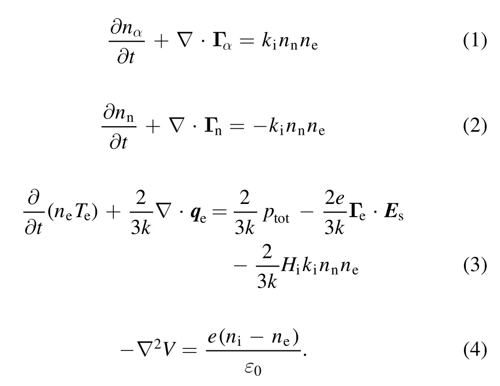
In the above equations,n α,Dα,and Γα(α=e, i,n)are the particle density, flux, diffusivity, and mobility, respectively.The neutral atom density was calculated bynn=2.41×1014pncm−3,wherepnis gas pressure, and its unit is Pa.Subscripts e, i, and n denote electrons, ions, and neutral atoms,respectively.Teis the electron temperature, and its unit is eV.Further,e,V,andε0are the elementary charge,potential,and the permittivity of free space, respectively.The electrostatic field corresponding to charge separation Esis given by the gradient of the potential, i.e.Es= −∇V·Hi=15.7 eV is the frist ionization energy,and the rate coefficient for ground state ionization is given by[44].The flux Γαin equation (1) is given by the modified drift-diffusion approximation:

where B0is the external static magnetic field, and μαis the mobility.We set a uniform background magnetic field along thezdirection, i.e.B0=B0ez.The electron mobilityμeand diffusion coefficientDeof electrons were calculated byandrespectively, where electron collision frequencyνeis given byνe=νen+νei[19].νenandνeiare the collision frequency between electrons and neutral atoms,and that between electrons and ions.

where Λln is the Coulomb logarithm, andσenis the collisional cross section between electrons and neutral atoms.

Equation (5) includes three-component equations and three-component unknowns.We can solve equation(5)using the following equations

Adopting the ambipolar diffusion approximation to parallel fluxes, equation (10) becomes

The flux of neutral atoms only takes into account the diffusion term in equation (2)

In equation(3),the influence of the magnetic field on the transport of electron temperature is neglected in the calculation of energy fluxqe

ptotis the electron power absorption, given as follows:

The plasma currentJpand the induced electric fieldEmfare calculated by Maxwell’s equations.

2.2.Maxwell’s equations

The high-frequency electric fieldEmfand the induced magnetic fieldBpwere calculated by Maxwell’s equations and the evolution equation of the plasma current, as follows:

whereme,μ0,andεrare the electron mass,the permeability of free space, and the relative permittivity of free space,respectively.Jais the antenna current, given by

Sais the cross-sectional area of the antenna,andIais the current amplitude.The total input power is generated from the electron power absorption corresponding to the plasma and the Joule heat of the antenna.The current amplitudeIawas adjusted to the electron power absorption to maintain a constant total power.Plasma currentJpis generated from the electron current.Therefore,equations(21)–(23)also represent the motion of electrons.

Figure 2.Discharge configuration (not to scale).

2.3.Initial conditions

The initial conditions in the simulation are as follows:

Reference [43] and the PHD simulations showed that the steady states were independent of a certain range of plasma density.However, the initial plasma densities must be large(about 1010cm−3)at the conditions of low pressure and strong magnetic field.Otherwise, the plasma density does not increase.This large plasma density value adopted within the experiment can be attributed to the capacitive mode,which was not considered in PHD.Another important aspect was the setting of the initial condition of the electromagnetic fields.We calculated the‘intrinsic’structures ofEmfandBpfor the initial plasma density and set them as the initial conditions.We setEmf=Bp=0and then calculated Maxwell’s equations for 20 radio frequency (RF) cycles before the discharge processes began, i.e.the plasma states were maintained to be the same,includingne,ni,andTe.Our evaluations showed that this method leads to convergence in a small amount of time,whereas using other initial conditions leads to divergence.

2.4.Discharge configuration and boundary conditio n

Figure 2 shows the discharge configuration.The boundary of the vacuum chamber is atr0=0.075 m,and the aluminum shield is atR0=0.125 m.The positions of the single-loop antenna with a width of 10 mm in the radial direction and 30 mm in the axial direction arera=0.09 m andza=0.3 m,respectively.This discharge configuration is roughly identical to the plasma source region of PPT.

The boundary conditions are as follows.

Table 2.Simulation parameters and constants.

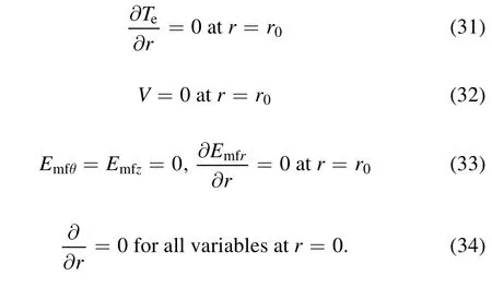
We only considered the discharge processes in the plasma source region.To reduce the impact of the boundary,the periodic boundary condition was employed for all variables in thezdirection.

2.5.Numerical methods

For fluid equations (1)–(3), we used a staggered grid in space,that is, scalars occupied a complete grid point, and vectors occupied half a grid point.Central difference was adopted in spatial discretization.The time discretization was in a fully implicit format and solved by successive over relaxation(SOR).

We also used central differences in spatial discretization for Poisson’s equation (4) and solved it by SOR.To overcome the limitation of the time step, a semi-implicit method was used to solve for the electric potential[45,46].The main idea of this method is to obtain the predicted electric field at the next time step using the electric field and plasma density distributions at the current time step.

The finite-difference time-domain method was used for equations (15)–(23).We used Yee’s staggered grid [47] in space discretization and solved the time discretization using the two-step alternating implicit format method.

3.Comparison of PHD with COMSOL and PPT

This section has two parts.A simple benchmark comparison was made between PHD and COMSOL Multiphysics software.for the case without the background magnetic field.Further, the results of PHD code are compared with the experimental results of PPT.Unless otherwise mentioned,the simulation parameters and constants were taken from table 2.

Figure 3.The temporal evolution of maximum ne.

Table 3.Simulation parameters.

3.1.Benchmark with COMSOL

COMSOL is a commercial software that is widely used for many scientific simulations.Considering that its inductively coupled plasma module is reliable and the results obtained with a background magnetic field are not widely known, we established a benchmark using this module.The simulation parameters are shown in table 3.To make the simulation conditions closer to those of COMSOL,we considered a series of chemical reactions involving metastable atoms[43,48,49]consistent with COMSOL.The boundary condition of the axial end plates was set the same as that for the side wall, and the electron collision frequencyνewas also set the same as that in COMSOL.

Figure 3 shows the evolution of electron density over time.The temporal evolution ofnecalculated by PHD is very similar to that obtained via COMSOL.The shapes of the steady-state structures of electron density are also similar;moreover,they are even more similar when the color bars are adjusted to a similar range, as figures 4(a) and (b) show.Both radial positions of the maximum plasma density are at the axis,and the axial positions are the same as the antenna position.The plasmas are mainly located near the antenna.

We further compare the radial distribution of electron density at =z0.3 m, as shown in figure 4(c).The maximum electron density obtained using COMSOL is×9.88 1011cm−3, whereas that obtained using PHD is 1.05×1012cm−3.The difference is about 6%, which is tolerable within discharge processes.

3.2.Comparison between PHD simulations and PPT experiments

Figure 4.Steady-state structure of ne in cm−3(at t=2000 Trf,Trf=7.37 × 10−8 s is the RF cycle),simulated by(a)PHD and(b)COMSOL,(c) the radial structures of electron density ( z =0.3 m).

Figure 5.The dependence of maximum ion density on (a) power P0 ,(b) gas pressure pn,and (c) magnetic field B0.

We compare the results of the present PHD simulation with those of prior PPT experiments.It should be noted that the experimental plasma density could only be evaluated in the diffusion zone in the PPT experiments, whereas PHD simulated only the source zone to save computing resources.Figure 5 shows the dependence of maximum ion density on(a) powerP0, (b) gas pressurepn,and (c) magnetic fieldB0.The magnitudes of the simulated and experimental values are similar, and their trends are consistent with each other.

For the pressure curve,the agreement is good below 0.6 Pa.For pressures above 0.6 Pa,the trend deviates signifciantly.The reason may be that as the pressure increases, the difference of plasma density between the source region and diffusion region increases.In general,the simulation results are consistent with the experiment qualitatively, and the quantitative comparison does not indicate a good similarity.This could be related to the simplifeid confgiuration of the simulation, the use of several assumptions to develop the model, the selection of boundary conditions, etc.

For the magnetic field curve, the deviation between the PHD and PPT seems to be getting large for the strong magnetic feild.The possible reasons are as follows.(1)The main losses of particles in the PPT experiment are sidewalls and end plates, and only the sidewalls are considered in the PHD simulation.(2) Classical diffusion is used in the simulation and the transport of particles may be slower than the experimental results.Thus, the loss of particles becomes smaller and the plasma density becomes larger.(3) The diagnostic location is far from the source and thus carries a certain amount of variation.In addition, the error in the diagnosis of Langmuir probes under strong magnetic fields may become larger.

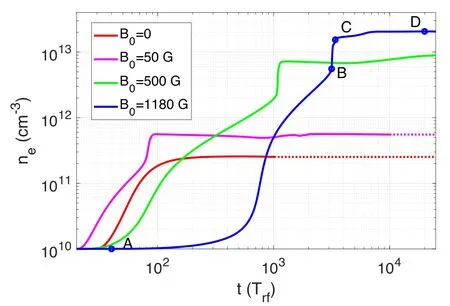
Figure 6.The temporal evolution of maximum ne for different B0 .

To sum up, the growth processes and the profiles of electron density are similar in the two simulations,and the numerical difference is small.Thus, the PHD code is reliable to a certain extent.

4.Discharge processes with varying background magnetic field

This section focuses mainly on the studied discharge processes without and with various magnetic fields.The discharge cases are executed atP0=2000 W,pn=0.35 Pa,and 0 ≤B0≤1180 G.The electron densities undergo linear growth and nonlinear saturation and finally attain the steady state,as shown in figure 6.It can be seen that the stronger the background magnetic field,the higher the steady-state plasma density.Interestingly, we discovered that density increased rapidly before reaching the steady state in the presence of magnetic field.We called it the second density jump,which is similar to the mode transition in helicon plasmas.The second density jumping time for the case ofB0=1180 G is approximatelyt=3000Trf.The electron density atB0=1180 G is about 82 times that without a magnetic field.Here are two possible explanations.First, there could be a resonant plasma density which is a function of magnetic fieldB0and gas pressurepn.The electromagnetic waves and the plasmas attain resonant states at this specific plasma density.This resonance results in high electron power absorption.Second, the magnetic field suppresses the plasma transport,which causes a reduction in the loss of plasma on the wall.Thus,the plasma density increases.However,the exact origin of the second density jump remains unclear.

Figure 7 shows the steady-state structure ofne.As the magnetic field increases, the uniformity of the axial distribution increases,and the plasma gradually diffuses from the local area to the entire vacuum area.

Figure 8 shows the periodically averaged distribution of the electron temperatureTeand the electron power absorptionPtotat the steady state.The negative values ofPtotmeans the electrons lose energy and the energy of the electrons is converted to the wave energy.Here, the manner in which the discharge occurs is briefly discussed.The electron power absorption increases the electron temperature; thus, the ionization cross-section becomes larger, and then, a large number of ionization processes are generated.A steady state is attained if the source terms balance the plasma loss.As the magnetic field increases, the electron temperature decreases.The axial position of maximalTeis the same as that of the antenna, except in the case ofB0=50 G.In addition,the maximal electron power absorption occurs near the central axis in the cases with a magnetic field,whereas it appears near the boundary in the case without a magnetic field,as shown in figure 8(b).The high temperature region near the antenna or near the source wall has been observed in the helicon thruster configuration[50–54].The PHD simulation results reproduce this phenomenon to some extent.Another interesting phenomenon is that the region of electron power absorption changes from one peak to two peaks in thezdirection when a magnetic field is introduced.With careful observation, we found that the number of radial patterns increases as the magnetic field increases.This is explained as follows.

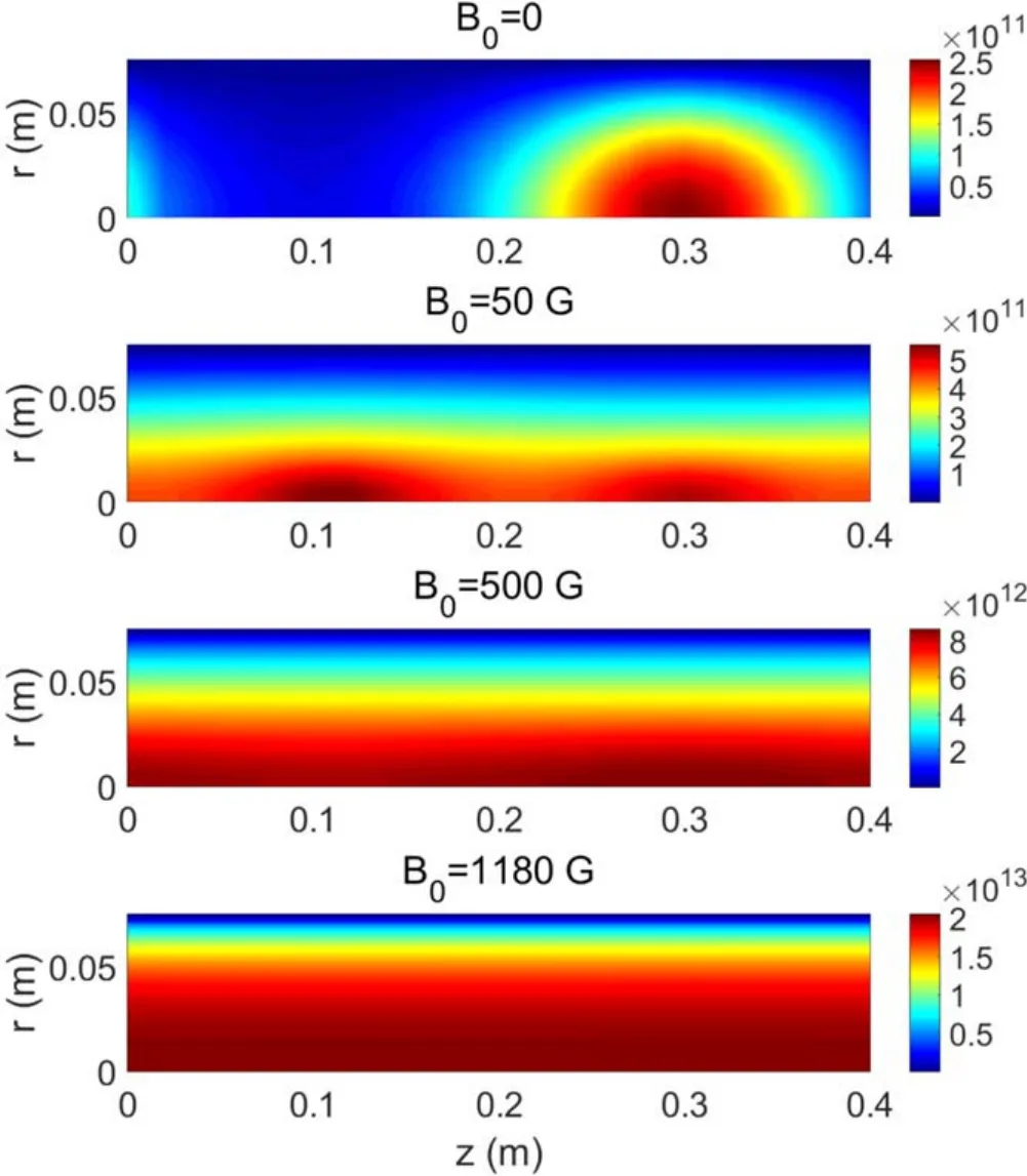
Figure 7.Steady-state structure of ne in cm −3.

It is usually considered that the helicon waves can propagate to the central axis owing to the weak damping rate.The periodic boundary conditions are likely to yield standing wave solutions.Standing helicon waves were also observed in the experiment[55–57].Thus,we speculated that the primary waves are standing helicon waves in these systems.Figure 9 shows the amplitude of the polar electric fieldθEmfand the induced magnetic fieldB zp at different moments.The amplitude ofθEmfdecays from the antenna position at the initial moment ( =tT40rf).When the second jump ( =tT3160rf)and the third jump ( =tT3400rf) being triggered, it becomes a standing wave structure and the amplitude in the plasma is higher than the antenna position.However,the electric field is not an obvious standing wave structure at steady state( =tT20000rf), which may be the reason why the results of high standing wave ratio(expressed as maxθEmf/minθEmfin plasmas) are not easily measured in experiments.The standing helicon waves yield the two axial and central peaks of electron power absorption.A larger magnetic field results in a higher density.The higher the density, the shorter the radial wavelength.Thus, the number of radial patterns increases.

From figures 6–8, it is clear that the obtained results show a reasonable relationship among electron density,electron temperature, and electron power absorption.The simulation results are consistent with the discharge law.

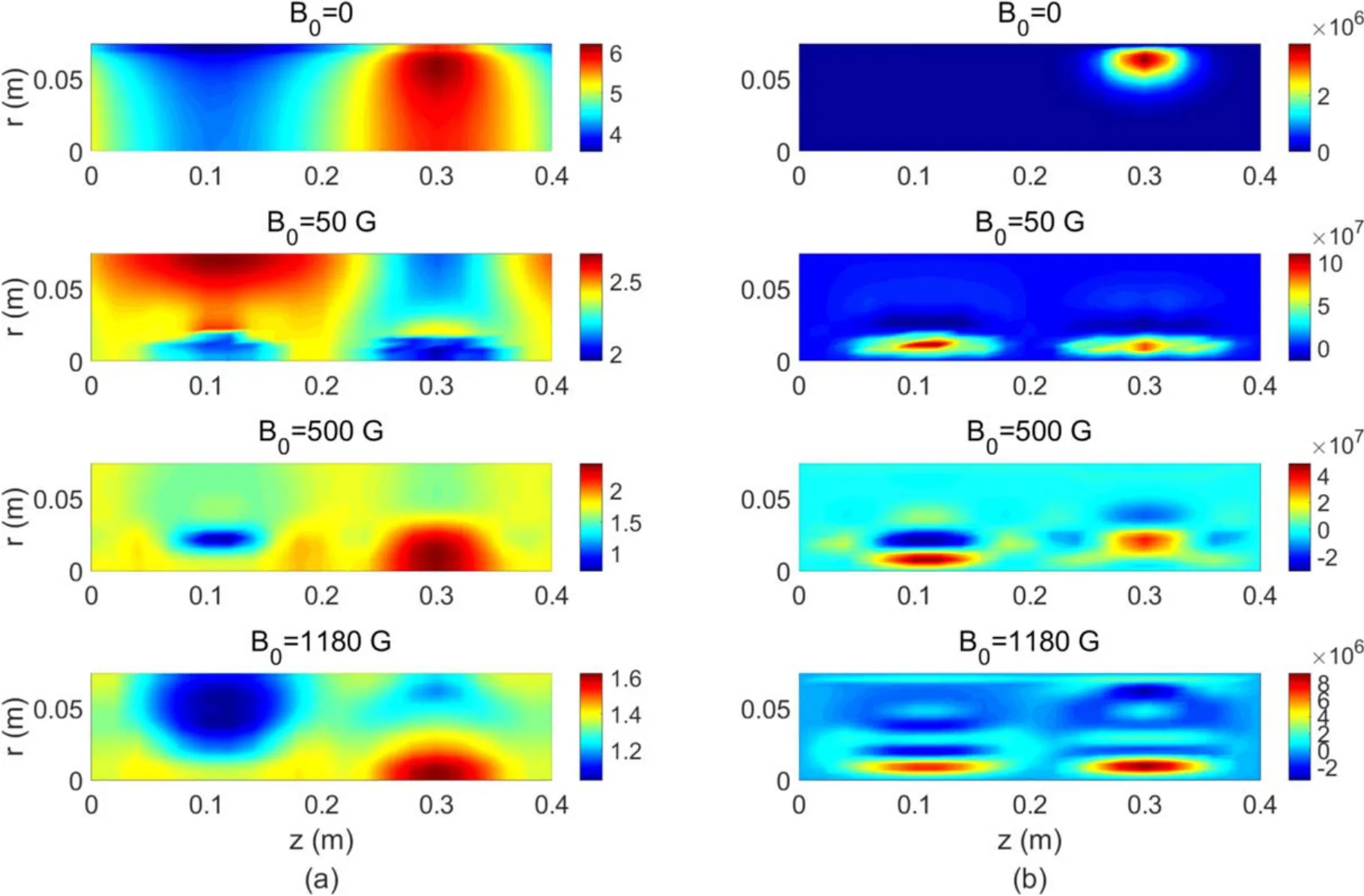
Figure 8.Cycle-averaged structure of (a)Te in eV and (b) the electron power absorption Ptot in W m−3 at steady state.

Figure 9.The amplitude of(a)the polar electric field Emfθin V m−1 and(b)the induced magnetic field Bpzin T at different moments for the cases of(2000 W,0.35 Pa,1180 G),where t=40 Trf ,t=3160 Trf ,t=3400 Trf and t=20000 Trf correspond to the points A,B,C,D in figure 6, separately.

5.Discussion and conclusions

In this study,a two-fluid discharge model that includes electron power absorption,ionization processes,and transport processes is established and employed to obtain numerical solutions.The PHD code can be used to simulate discharge processes under a low pressure (～0.5 Pa) and strong background magnetic field(～1 kG).The results obtained in the absence of a magnetic field are in reasonable agreement with those obtained using COMSOL, and the results obtained under the typical helicon discharge parameters generally conform to the law governing the discharge processes.The results of the scanning parameters are consistent with the experimental results qualitatively but not quantitatively.Compared with that in the case of no background magnetic field, the plasma density under a strong magnetic field is an order of magnitude higher, which is consistent with the discharge law that was verified experimentally.The maximal electron power absorption in the steady state occurs near the central axis in the presence of the magnetic field.It could be due to the standing helicon waves.The second density jumps were discovered in the complete discharge processes.These results may help us understand the discharge mechanism.Particularly,the occurrence of steady-state density jumps with an increase in power is an important result.However, thorough results could not be obtained because the plasma loss is insufficient owing to the application of periodic boundary conditions.This was a limitation of this study.In general, the simulation in this study is preliminary and needs further investigation in terms of boundary conditions,discharge configuration, vertical temperature transport, symmetry breaking, antenna optimization, metastable atom reactions, etc.

Acknowledgments

We are grateful to Professor Younian Wang and Shuxia Zhao from Dalian University of Technology, who have provided substantial assistance for the establishment of the model.This work was supported by National Natural Science Foundation of China (No.11975038).