
ZERO KINEMATIC VISCOSITY-MAGNETIC DIFFUSION LIMIT OF THE INCOMPRESSIBLE VISCOUS MAGNETOHYDRODYNAMIC EQUATIONS WITH NAVIER BOUNDARY CONDITIONS∗
2021-10-28 05:44FucaiLI栗付才
Fucai LI(栗付才)
Department of Mathematics,Nanjing University,Nanjing 210093,China
E-mail: fli@nju.edu.cn
Zhipeng ZHANG(张志朋)†
Department of Mathematics,Nanjing University,Nanjing 210093,China;Institute of Applied Physics and Computational Mathematics,Beijing 100088,China
E-mail:zhangzhipeng@nju.edu.cn
Abstract We investigate the uniform regularity and zero kinematic viscosity-magnetic diffusion limit for the incompressible viscous magnetohydrodynamic equations with the Navier boundary conditions on the velocity and perfectly conducting conditions on the magnetic field in a smooth bounded domain Ω⊂R3.It is shown that there exists a unique strong solution to the incompressible viscous magnetohydrodynamic equations in a finite time interval which is independent of the viscosity coefficient and the magnetic diffusivity coefficient.The solution is uniformly bounded in a conormal Sobolev space and W1,∞(Ω)which allows us to take the zero kinematic viscosity-magnetic diffusion limit.Moreover,we also get the rates of convergence in L∞(0,T;L2),L∞(0,T;W1,p)(2≤p<∞),and L∞((0,T)×Ω)for some T>0.
Key words incompressible viscous MHD equations;ideal incompressible MHD equations;Navier boundary conditions;zero kinematic viscosity-magnetic diffusion limit
1 Introduction
We consider the incompressible viscous magnetohydrodynamic(MHD)equations(for example,see[6,9])

in(0,T)×Ω,where Ω⊂R3is a smooth bounded domain.The unknowns v∊,H∊and p∊represent the velocity,the magnetic field and the pressure of the fluid,respectively.The pressure p∊can be recovered from v∊and H∊via an explicit Calder´on-Zygmund singular integral operator([7]).Here,we assume that the viscosity coefficient is equal to the magnetic diffusivity coefficient,denoted by∊>0.We add to system(1.1)the initial-boundary conditions
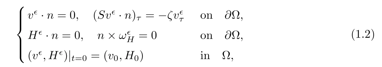
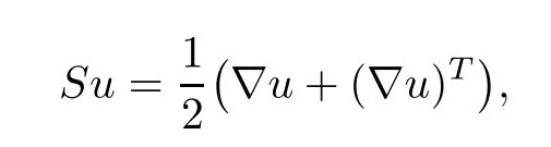
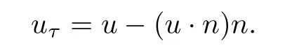
where(∇u)Tdenotes the transpose of the matrix∇u,and uτstands for the tangential part of u on∂Ω,i.e.,
The boundary condition(1.2)1was first introduced by Navier in[18]to show that the velocity is proportional to the tangential part of the stress;it allows the fluid slip along the boundary and is often used to model rough boundaries.The boundary condition(1.2)1can be generalized to the following form([11]):

Here A is a(1,1)-type tensor on the boundary∂Ω.When A=ζ Id(Id denotes the identity matrix),(1.3)is reduced to the standard Navier boundary conditions.In addition,for smooth functions,we can get the form of the vorticity

where ω=∇×u and B=2A−S(n)(see[27]).
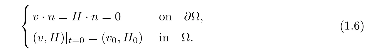
In this paper,we are interested in the uniform regularity and the zero kinematic viscositymagnetic diffusion limit of the problem(1.1)–(1.2),and taking the limit∊→0 to obtain the ideal incompressible MHD equations(Suppose that the limits v∊→v and H∊→H as∊→0 exist),i.e.

with the following initial-boundary conditions:
When taking H∊=0 in the system(1.1),it is reduced to the classical incompressible Navier-Stokes equations.There are a lot of works on the vanishing viscosity limit of the incompressible Navier-Stokes equations.The inviscid limit of the Cauchy problem has been studied by many authors,see[14,16,21].When the boundary appears,the inviscid limit problem becomes challenging due to the possible appearance of the boundary layer[13,19].On one hand,for the incompressible Navier-Stokes equations with no-slip boundary condition,its vanishing viscosity limit is wildly open except when the initial datum is analytic[22,23]or the initial vorticity is located away from the boundary in the two-dimensional half plane[15].On the other hand,considering the incompressible Navier-Stokes system with Navier boundary conditions,more results are available,see[2–5,11,13,17,28]and the references cited therein.The uniform H3bound and a uniform existence time interval with respect to∊were obtained by Xiao and Xin[28]for the flat boundary.Subsequently,the conclusions in[28]were extended to Wk,p(Ω)with k≥3 and p≥2 in[2].The main reason for this is that the boundary integrals vanish on the flat boundary,see also[3,4].However,such results can’t be expected for the general boundary since boundary layer may appear.In order to analyze the effect of the boundary layer in a general bounded domain,Iftimie and Sueur[13]constructed the boundary layer for the incompressible Navier-Stokes equations with the Navier boundary condition(1.2)1in the form

where the function V vanishes for x outside a small neighborhood of∂Ω and φ(x)is the distance between x and∂Ω for x in a neighborhood of∂Ω.The boundary layers constructed in[13]are of width O(√∊),like the Prandtl layer[19],but are of amplitude O(√∊)(the Prandtl layer is of width O(√∊)and of amplitude O(1)).Thus it is impossible to obtain the H3(Ω)or W2,p(Ω)(p large enough)uniform estimates for the incompressible Navier-Stokes equations.Recently,Masmoudi and Rousset[17]considered the vanishing viscosity limit for the incompressible Navier-Stokes equation with the boundary condition(1.2)1in the anisotropic conormal Sobolev spaces(de fined below),and this can eliminate the effects of normal derivatives near the boundary.They obtained uniform regularity and the convergence of the viscous solutions to the inviscid one by compactness arguments.Subsequently,some results in[17]were extended to the compressible isentropic Navier-Stokes equations with Navier boundary conditions[20,26].Moreover,based on the results in[17],the rates of convergence in different spaces were obtained by Gie and Kelliher[11]and Xiao and Xin[27],respectively.
As for the 3D incompressible viscous MHD equations,the study of the inviscid limit is quite limited,see[29–31].Specially,Xiao,Xin and Wu[29]investigated the inviscid limit for the system(1.1)with the boundary conditions
Motivated by[17],in this paper,we investigate the inviscid limit for the system(1.1)with Navier boundary conditions for(u∊,H∊)in a bounded domain Ω⊂R3in the framework of anisotropic conormal Sobolev spaces.Due to the strong coupling between v∊and H∊,a priori estimates become more complicated than that in[17].We obtain the uniform regularity of the solution,which allow us to pursue the inviscid limit for the problem(1.1)–(1.2).Moreover,we obtain some rates of convergence for(v∊,H∊)in different spaces.
Our uniform regularity result reads as follows:

Based on the uniform estimates in Theorem 1.1,by strong compactness arguments similar to those of[17],we can justify the zero kinematic viscosity-magnetic diffusion limit,but without a convergence rate.In what follows,we are interested in the zero kinematic viscosity-magnetic diffusion limit with rates of convergence.First,thanks to the result in[24],we know that there exists a unique solution(v,H)∈H3of the ideal incompressible MHD equations(1.5)with the boundary condition(1.6)1and the initial condition(v0,H0)∈H3which satis fies
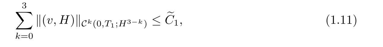
Theorem 1.3Assume that(v0,H0)belong to H3(Ω)and satisfy the same assumptions as in Theorem 1.1.Let(v,H)be the smooth solution of(1.5)–(1.6)on[0,T1],and(v∊,H∊)be the solution of(1.1)–(1.2)on[0,T0].Then there exists a time T2=min{T0,T1}>0 and a constantsuch that
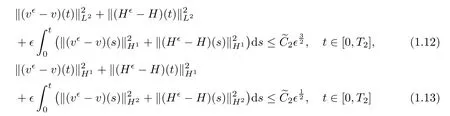
for∊small enough.Consequently,

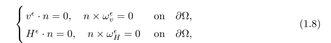
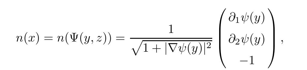
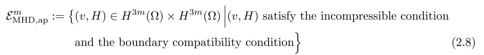
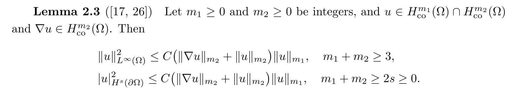
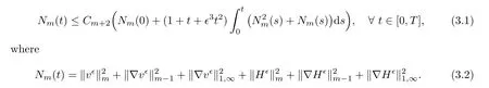
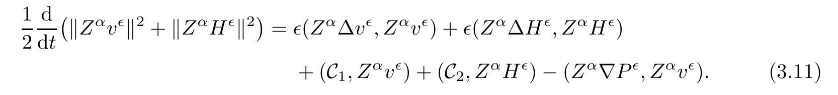
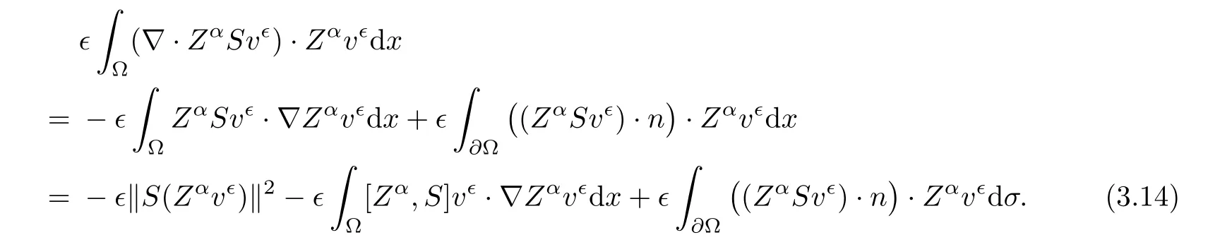
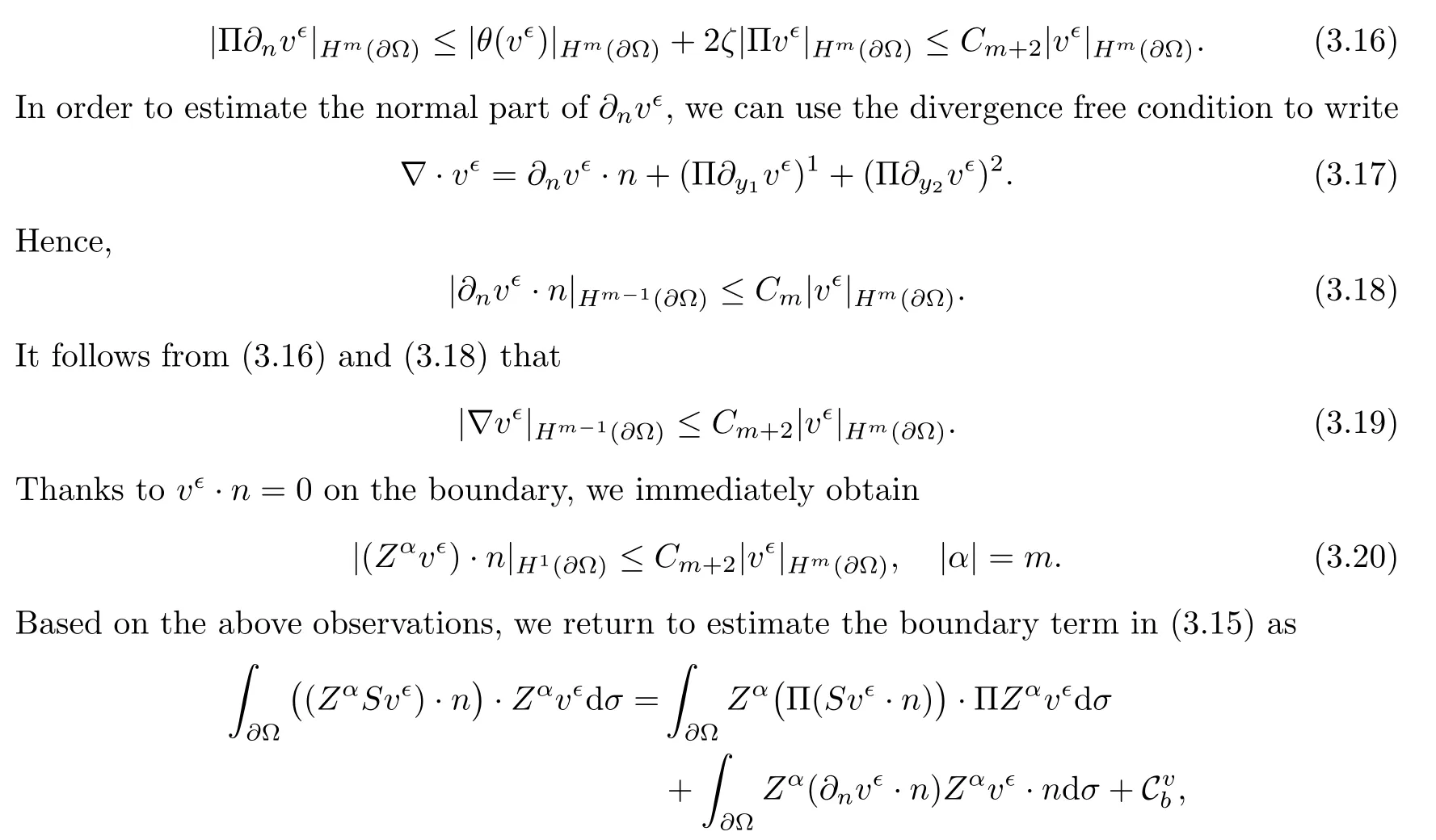
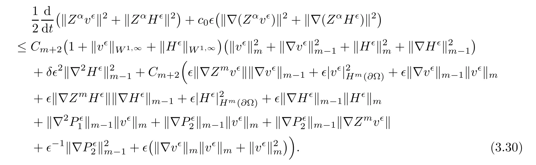
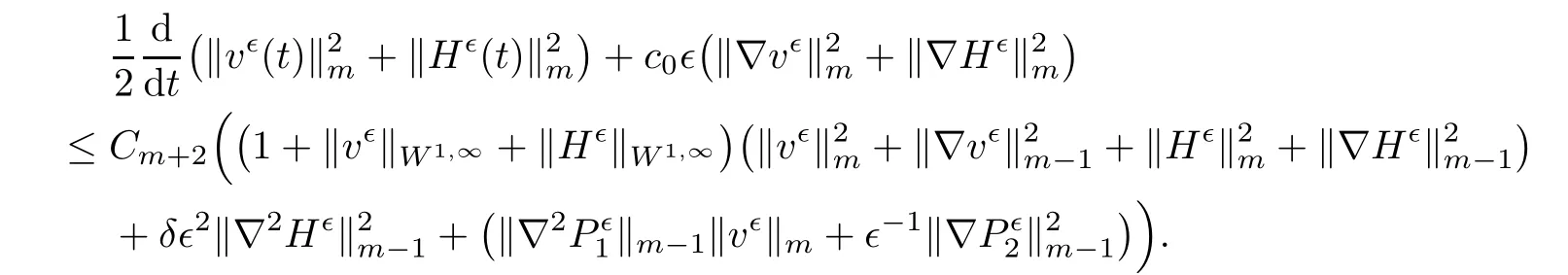
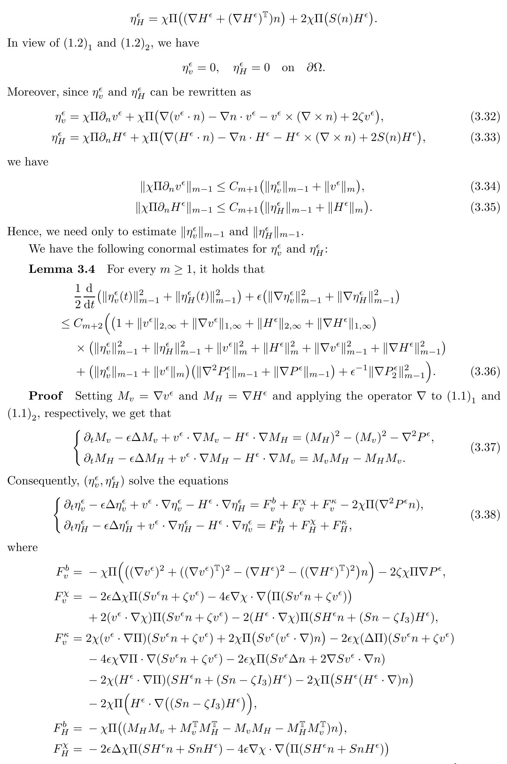
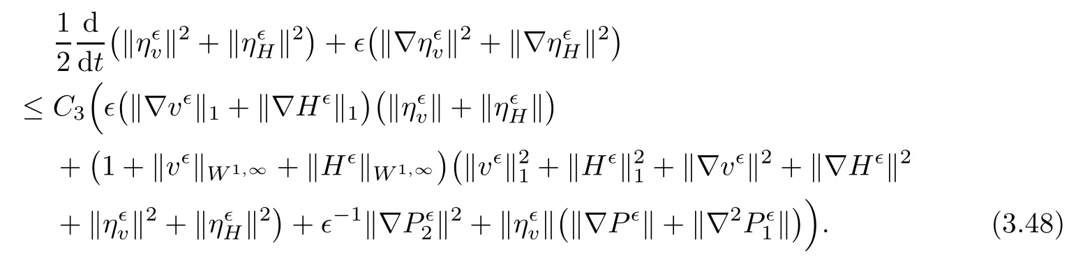
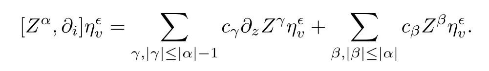
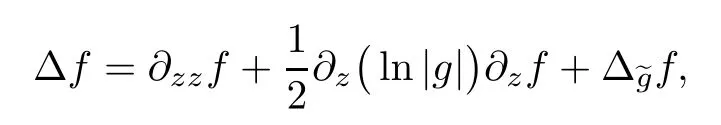
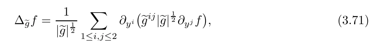
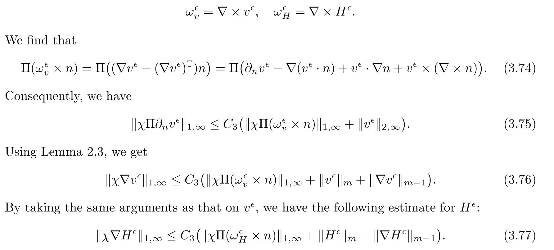
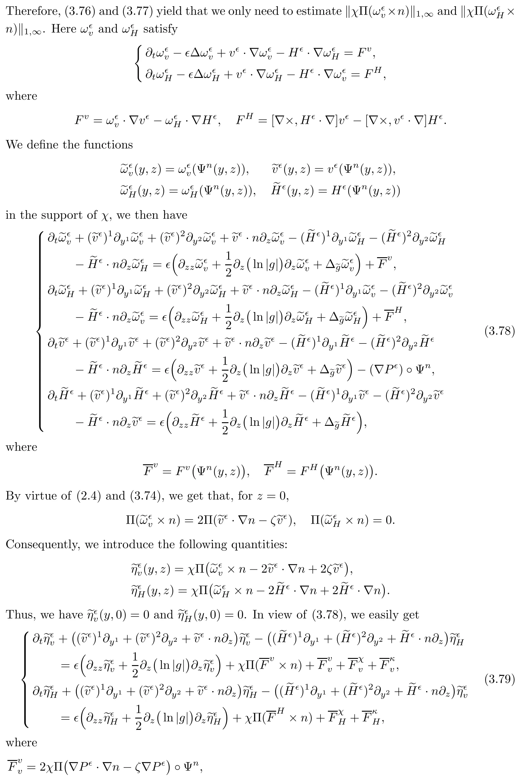
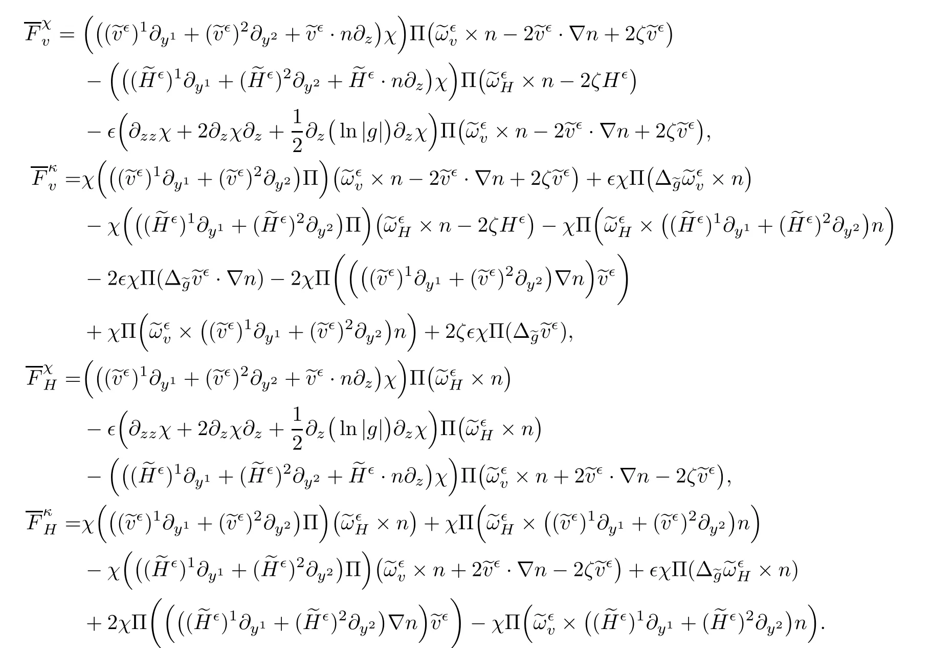
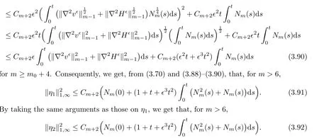
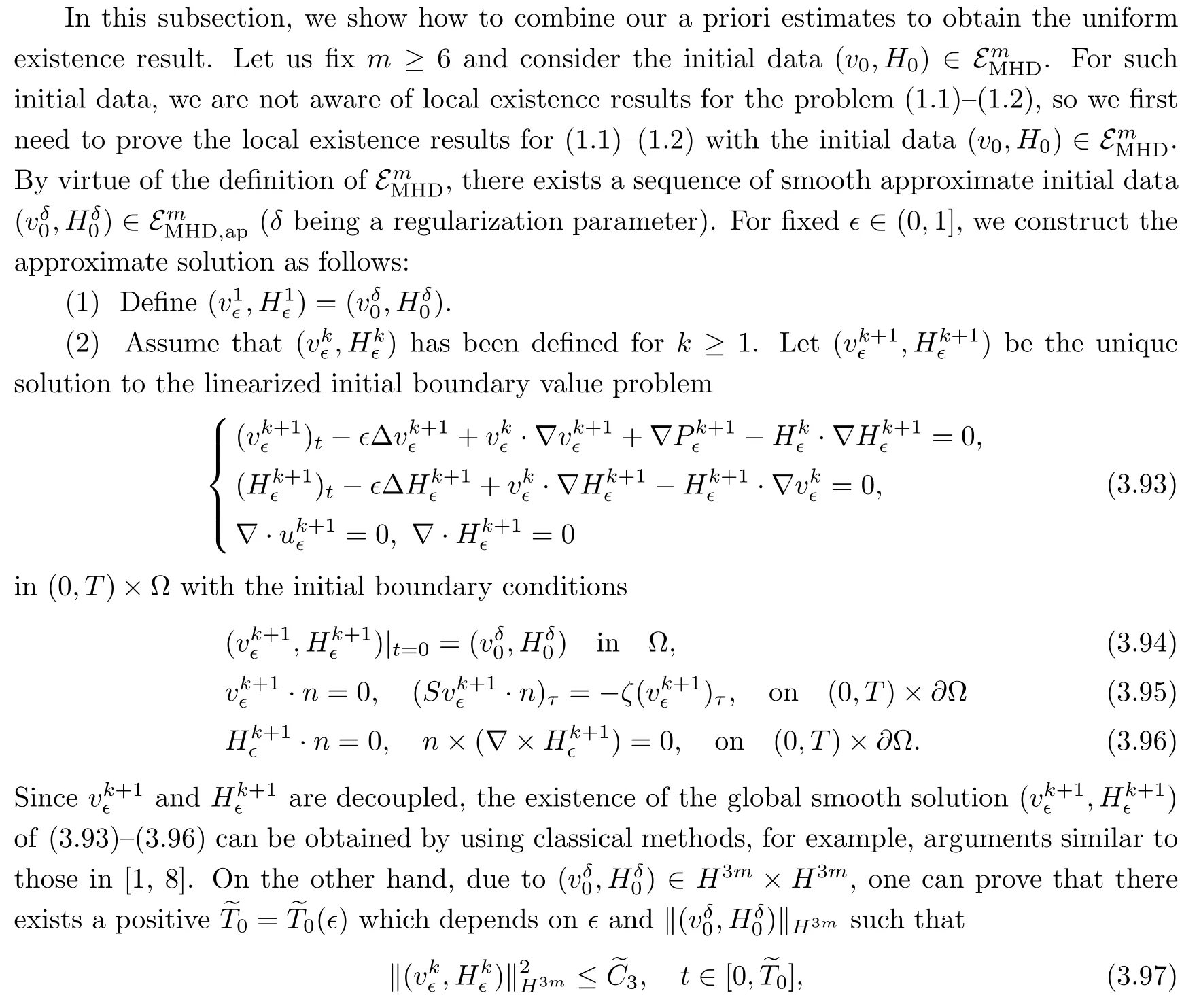
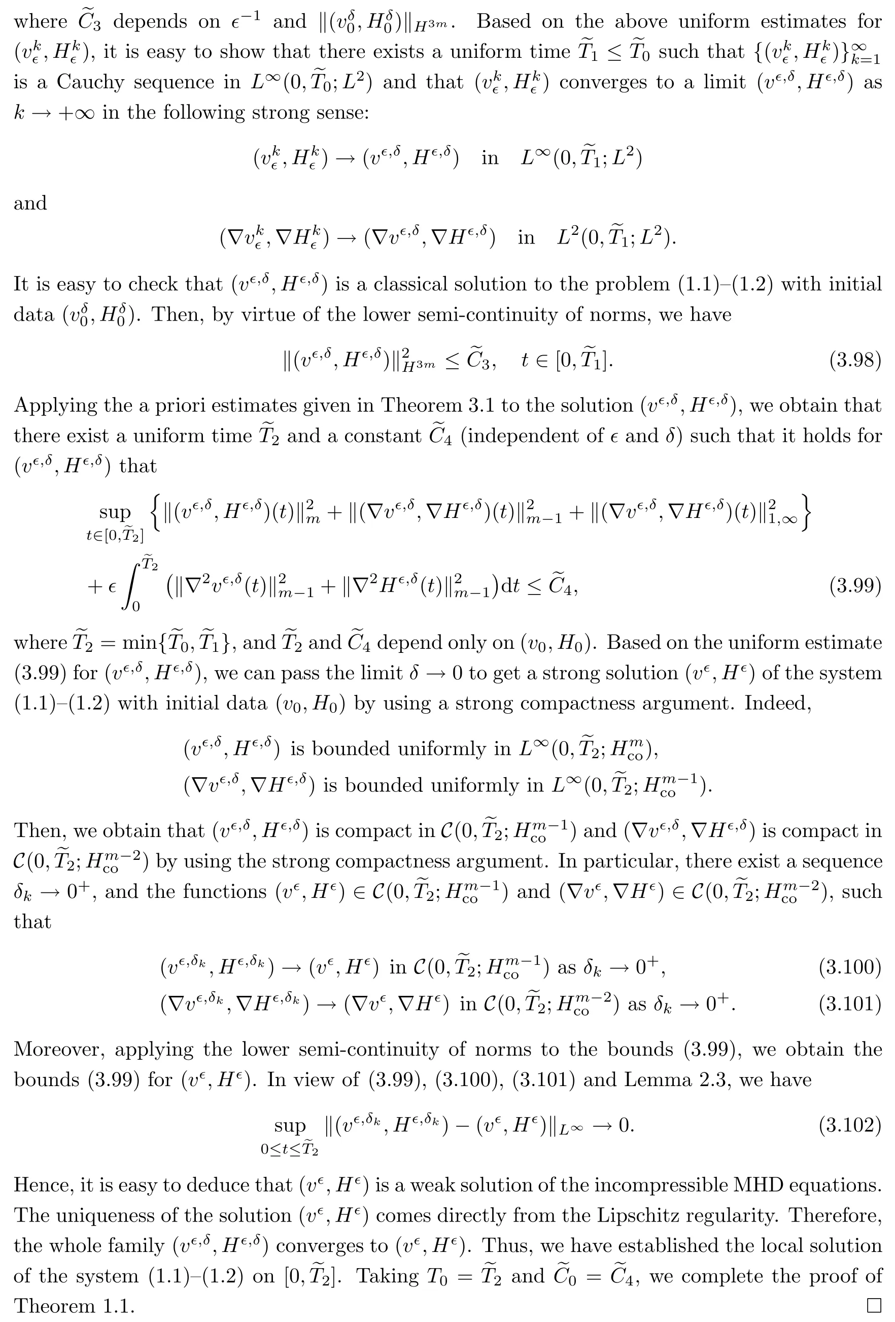
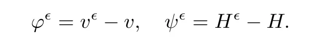
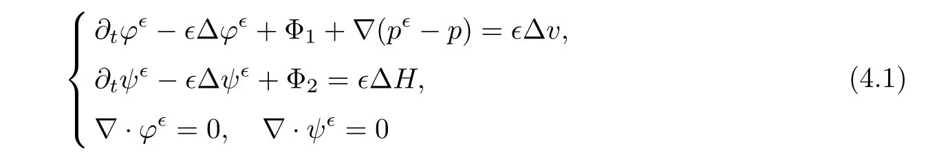
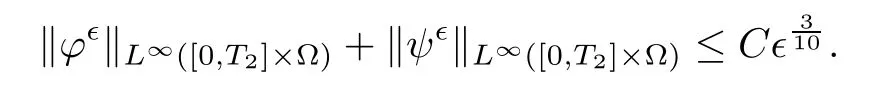
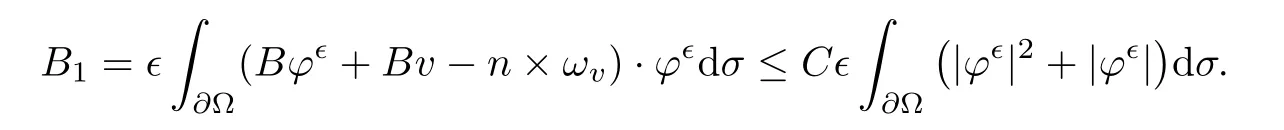
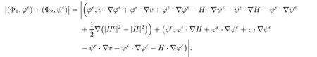
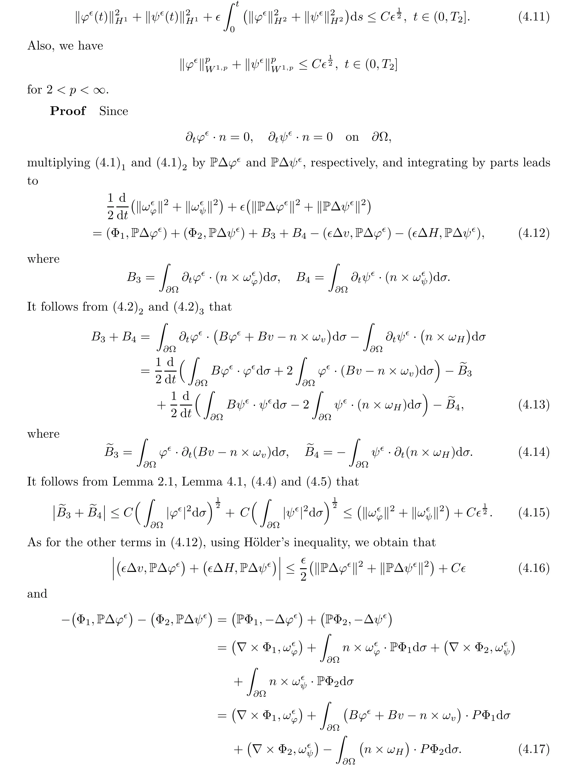
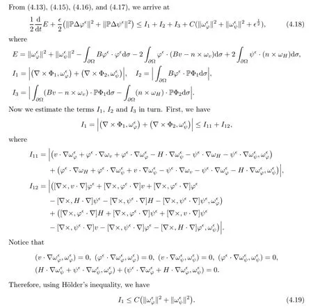
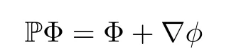
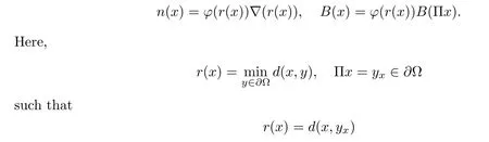
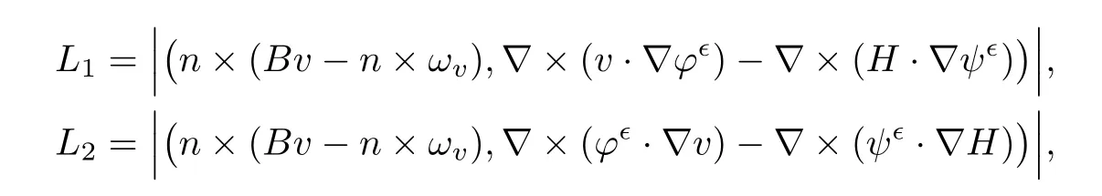
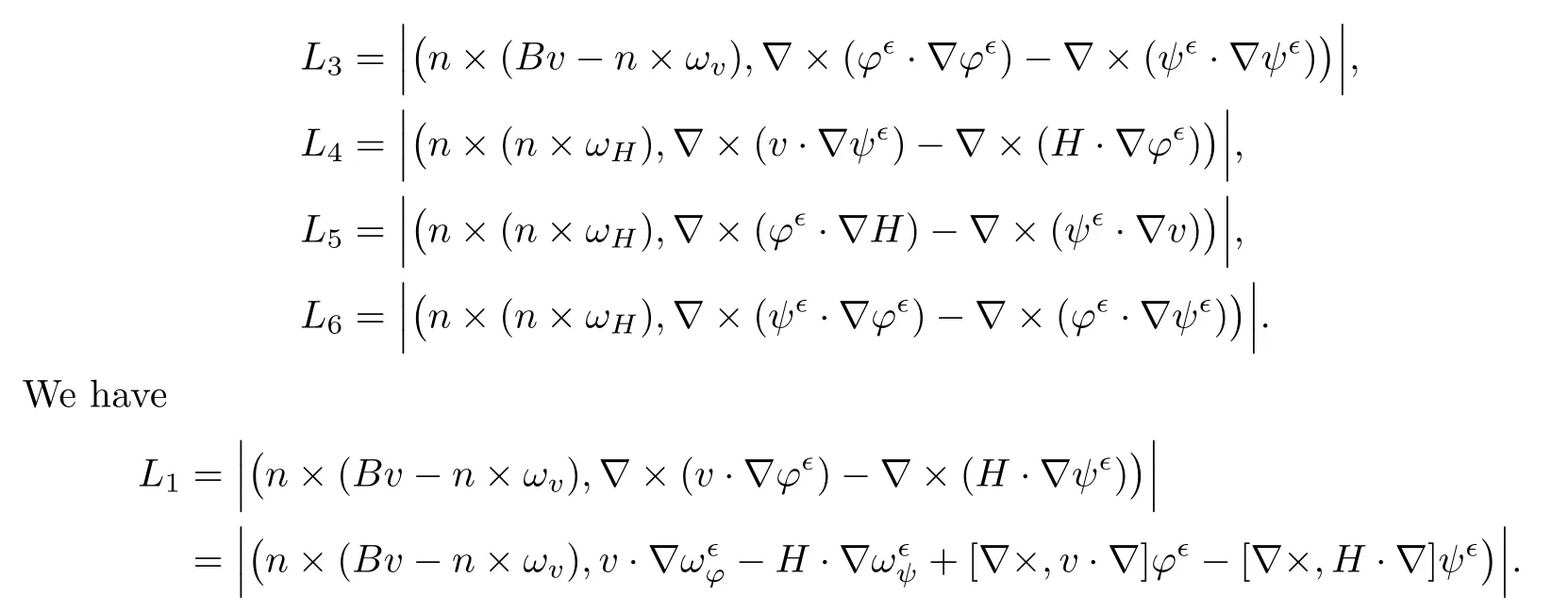
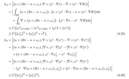
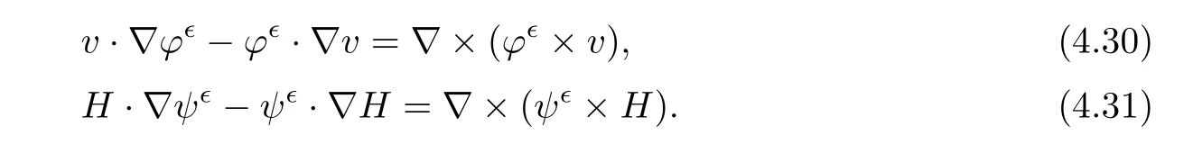
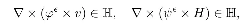
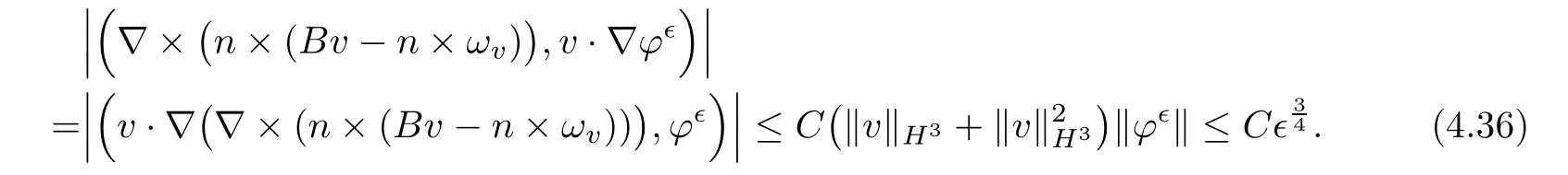
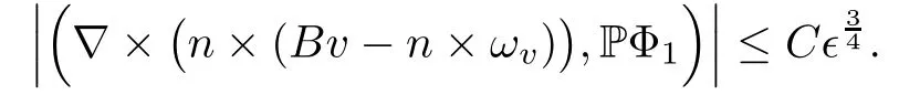
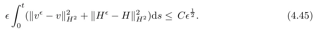
for 2 We now outline the proof of Theorem 1.3.Our approach is similar to that of[27]in spirit.However,due to the strong coupling between the magnetic field and the velocity field,we meet some new difficulties.We first give the rates of the convergence in L∞(0,T2;L2(Ω))and L∞([0,T2]×Ω)by using an elementary energy estimate and Gagliardo-Nirenberg interpolation inequality.Next,we find that it is very difficult to estimate some boundary terms caused by multiplying(4.1)1by∆(v∊−v)and(4.1)2by∆(H∊−H)directly in the proof of the rate of the convergence in L∞(0,T2;H1(Ω)).Indeed,we get‖v∊‖H2≤‖P∆v∊‖+‖v∊‖and‖H∊‖H2≤‖P∆H∊‖+‖H∊‖from Section 2 in[27],where P is Leray projector.Therefore,we replace∆(v∊−v)and∆(H∊−H)by P∆(v∊−v)and P∆(H∊−H)to prove the rates of the convergence in L∞(0,T2;H1(Ω))and L∞(0,T2;W1,p(Ω)). The rest of this paper is organized as follows:in the next section,we give some assumptions on the domain and the de finitions on conormal Sobolev spaces,and present some inequalities which will be used frequently.In Section 3,we prove a priori energy estimates and give the proof of Theorem 1.1.Theorem 1.3 will be veri fied in Section 4. Throughout this paper,we shall denote by‖·‖Hmand‖·‖W1,∞the usual Sobolev norms in Ω and‖·‖for the standard L2norm.The letter C is a positive constant which may change from line to line,but which is independent of∊∈(0,1]and|ζ|≤1. We first state the assumptions on the bounded domain Ω⊂R3and then introduce some norms.We assume that Ω has a covering such that We say that Ω is Cmif the functions ψkare Cmfunctions.Denote by Cma positive constant independent of∊∈(0,1]and|ζ|≤1 which depends only on the Ck-norm of the functions ψk,k=1,···,n. To de fine the conormal Sobolev spaces,we consider(Zk)1≤k≤N,a finite set of generators of vector fields that are tangential to∂Ω,and set In this paper,we shall still denote by∂i(i=1,2,3)or∇the derivatives with respect to the standard coordinates of R3.The coordinates of a vector field u in the basiswill be denoted by ui,thus, We denote by uithe coordinates in the standard basis of R3,i.e., Denote by n the unit outward normal vector which is given locally by and by Π the orthogonal projection Π(x)=Π(Ψ(y,z))u=u−n(Ψ(y,z)),which gives the orthogonal projector onto the tangent space of the boundary.Note that n and Π are de fined in the whole Ωkand do not depend on z.By using these notations,(1.2)1and(1.2)2read as where θ is the shape operator(second fundamental form)of the boundary,θ(v∊)=and θ(H∊)= Since the boundary layers may appear in the presence of physical boundaries,in order to obtain the uniform estimates for the solutions of the incompressible MHD equations with the boundary conditions(1.2)1and(1.2)2,we need to find a suitable functional space.Here,we de fine the functional space Em(T)for functions(v,H)(t,x)as where the norm‖(·,·)‖Emis given by We note that the a priori estimates in Theorem 3.1 below are obtained in the situation in which the approximate solution is sufficiently smooth up to the boundary.Therefore,in order to obtain a self-contained result,we need to assume that the approximated initial data satis fies the boundary compatibility conditions(1.2)1and(1.2)2.For the initial data(v0,H0)satisfying(1.6)2,it is not clear if there exists an approximate sequence(δ being a regularization parameter)which satis fies the boundary compatibility conditions and0 as δ→0.Thus,we set and Now we introduce some inequalities.First,we give a well-known inequality. Lemma 2.1([25,28]) For u∈Hs(Ω)(s≥1),we have Next,we introduce Korn’s inequality,which plays an important role in energy estimates. Lemma 2.2(Korn’s inequality[10]) Let Ω be a bounded Lipschitz domain of R3.There exists a constant C>0 depending only on Ω such that Third,we also need the following anistropic Sobolev embedding and trace estimates: Finally,we introduce the following Gagliardo-Nirenberg-Moser inequality,which will be used frequently: The main aim of this section is to prove the following a priori estimates which is the crucial step in the proof of Theorem 1.1.To this end,let(v∊,H∊)be the solution of the problem(1.1)–(1.2)with pressure p∊.Moreover,the solution(v∊,H∊,p∊)possesses proper regularity such that the procedure of formal calculations makes sense. Theorem 3.1For m>6 and a Cm+2bounded domain Ω,there exists a constant Cm+2>0,independent of∊∈(0,1]and|ζ|≤1,such that for any sufficiently smooth solution de fined on[0,T]of the problem(1.1)–(1.2)in Ω,we have Since the proof of Theorem 3.1 is quite complicated and lengthy,we divide it into subsections. In this subsection,we first give the basic a priori L2energy estimate. Lemma 3.2For a smooth solution to the problem(1.1)–(1.2),it holds that,for any∊∈(0,1]and|ζ|≤1, ProofMultiplying(1.1)1and(1.1)2by v∊and H∊,respectively,applying the boundary condition(1.2),and integrating by parts,we obtain where(·,·)stands for the L2scalar product.Now,let us treat the terms with the coefficient∊in(3.4).Integrating by parts and using the boundary condition(1.2)1,we have Putting(3.5)and(3.6)into(3.4),we then obtain(3.3). We remark that the above basic energy estimation is insufficient to get the vanishing viscosity limit.Thus,higher order energy estimates are needed. Lemma 3.3For every m∈N+,it holds that ProofIn view of Korn’s inequality and Lemma 3.2,we can prove the case for m=0.Now we assume that(3.7)has been proved for|α|≤m−1.We shall prove that it also holds for|α|=m≥1.Applying Zαwith|α|=m to(1.1)1and(1.1)2,respectively,we obtain that where Multiplying(3.10)1and(3.10)2by Zαv∊and ZαH∊,respectively,and integrating by parts,we have First,in view of Lemma 2.4,we obtain that Next,we deal with the terms with the viscosity coefficient∊.Notice that For the first term of the right-hand side of(3.13),by integrating by parts,we get Thus,it follows from Lemma 2.2 that there exists a c0>0 such that It remains to control the boundary term in(3.15).To this end,we have the following observations:due to the Navier boundary condition(2.4),we obtain To estimate the boundary term,we note that when m=1,(3.7)can be obtained easily.Thus we assume that m≥2.Integrating by parts along the boundary,we get Substituting(3.12),(3.26),(3.27)and(3.29)into(3.11),we obtain that Consequently,using Lemma 2.3,Young’s inequality,and the assumptions with respect to|α|≤m−1,we have This ends the proof of Lemma 3.3. In view of(3.31)and(3.32),we obtain Similarly,we get Furthermore,using(3.46),(3.47)and Young’s inequality,we have Since∊(‖∇v∊‖1+‖∇H∊‖1)has been estimated in Lemma 3.3,this yields(3.36)for the case of m=1. To prove the general case,we assume that(3.36)holds for|α|≤m−2.Let us consider the situation where|α|=m−1.Applying Zαto(3.38)1and(3.38)2,respectively,yields that where Multiplying(3.49)1and(3.49)2by Zαand Zα,respectively,and integrating by parts,we obtain that where i=1,2,3.To estimate the last two terms on the right-hand side of(3.51),we use the structure of the commutator[Zα,∂i]and the expansionin the local basis.We have the following expansion: We can do similar calculations for the other terms in C3and C4.Consequently,based on(1.2)1,(1.2)2and Lemma 2.4,we get By combining(3.50),(3.54)–(3.57)and(3.59)–(3.61),and using the induction assumption and Young’s inequality,we get(3.36). The aim of this subsection is to give the pressure estimates. Lemma 3.5For every m≥2,we have the following estimates: In order to enclose the estimates in(3.70),we need to control‖∇v∊‖1,∞and‖∇H∊‖1,∞.We have Lemma 3.6For m>6,it holds that ProofWe observe that,away from the boundary,the following estimates hold: Here{βi}is a partition of unity subordinated to the covering(2.1).In order to estimate the near boundary parts,we adopt the ideas of Proposition 21 of[17].We use a local parametrization in the vicinity of the boundary given by a normal geodesic system where We can extend n and Π in the interior by setting We observe∂z=∂nand Hence,the Riemann metric g has the following form: Consequently,the Laplacian in this coordinate system reads as where|g|is the determinant of the matrix g and∆~gis de fined by With these preparations,we begin to estimate the near boundary parts.In view of Lemma 2.3 and the equality(3.17),we have Hence,we need only to estimate‖χΠ∂nv∊‖1,∞and‖χΠ∂nH∊‖1,∞.To this end,we introduce the vorticity Note that in the derivation of the source terms above,we have used the fact that in the coordinate system just de fined,Π and n do not depend on the normal variable.Since∆~ginvolves only the tangential derivatives,and the derivatives of χ are compactly supported away from the boundary,the following estimates hold: A crucial estimate towards the proof of Lemma 3.6 is the following lemma: Lemma 3.7([17]) Let ρ be a smooth solution of where u satis fies the divergence free condition and u·n vanishes on the boundary.Assume that ρ and f are compactly supported with respect to z.Then Therefore,we complete the proof of Lemma 3.6. Based on Lemma 3.6 and(3.70),we can easily prove Theorem 3.1.We omit the details here. In this section,we study the zero kinematic viscosity-magnetic diffusion limit of viscous solutions to the inviscid one with rates of convergence in different spaces.For the convenience of calculations,we replace the boundary conditions in(1.2)by(1.10).De fine It then follows from(1.1)and(1.5)that ϕ∊and ψ∊satisfy in Ω×(0,T2)with the initial boundary conditions and 0 We start with the rates of convergence in L∞(0,T2;L2)and L∞([0,T2]×Ω). Lemma 4.1Under the assumptions in Theorem 1.3,it holds Furthermore,we have ProofMultiplying(4.1)1and(4.1)2by ϕ∊and ψ∊,respectively,and integrating the results by parts,we have Next,we deal with the boundary integrals B1and B2.For B1,we have In view of Lemma 2.1,the trace theorem and the interpolation inequality we further obtain that where δ is small enough.Similarly,we also get that Finally,we deal with(Φ1,ϕ∊)and(Φ2,ψ∊).We have Using(4.1)3,(4.2)2and(4.2)3,we have Consequently,we obtain Based on Lemma 2.1,(4.3),(4.6),(4.7)and(4.8),we arrive at Then,by using Gronwall’s inequality,we get that,for t∈(0,T2], Furthermore,using the Gagliardo-Nirenberg interpolation inequality,we have This completes the proof of Lemma 4.1. Next,we focus on proving the rates of convergence in L∞(0,T;H1)and L∞(0,T;W1,p)(2≤p<∞). Lemma 4.2Under the assumptions in Theorem 1.3,it holds Next,we estimate the term I2.It is well known that holds for any function Φ∈L2(Ω).Thus we only need to control the scalar function φ.However,it is difficult to estimate φ on the boundary∂Ω.In order to overcome this difficulty,we need to transform it to an estimate on Ω.First,we should extend n and B to the interior of Ω as follows: is well-de fined in Ωσ={x∈Ω,r(x)≤2σ}for some σ>0 and ϕ(s)∈[0,2σ)satisfying Then,by integrating by parts,we can obtain We easily get that As for the remaining terms in(4.20),by the same arguments as to those of I1,we have It follows from(4.21)and(4.22)that Finally,we deal with I3,i.e., We observe that the estimate is trivial if the system(1.5)satis fies the same boundary conditions as the system(1.1)does.In general,[Bv]τ−n×ωvand[BH]τ−n×ωHmay be not equal to zero.As a result,the boundary layer may occur,so we will experience more complicated estimates.Similarly to I2,we obtain that We first deal with the term I31.It follows from the de finitions of Φ1and Φ2that where We first deal with the terms which contain higher derivatives.Integrating by parts leads to Compared to L1,both L2and L3can be easily estimated.In fact,we have We find that L4,L5and L6have similar structures to those of L1,L2and L3,respectively,so we can get It follows from(4.24)–(4.29)that Now,it remains to estimate the term I32,i.e., We consider the first term in I32.Since it involves Leray projection,some terms which contain higher derivatives of ϕ∊or ψ∊cannot be estimated easily.We have the following observations: Furthermore,since ϕ∊·n=0,v·n=0,ψ∊·n=0 and H·n=0,we have where λ1and λ2are two scalar functions de fined on∂Ω.Based on the above observations,we easily obtain that where H is Leray projection space.Thus we have the equality Then it follows from(4.33),(4.34)and Lemma 4.1 that Next,by integrating by parts,we have Similarly,we obtain that In addition,we directly get that Therefore,in view of(4.35)–(4.38),we obtain that By taking the same arguments as to those above,we observe that Hence,we get which implies Thus,we conclude that In conclusion,it follows from(4.19),(4.23)and(4.41),that Now we need to deal with the left terms in the above inequality.Let us recall that In view of Lemma 2.1,we obtain where δ is small enough.Consequently,we get Applying Gronwall’s inequality to(4.42)gives us Thus,thanks to Lemma 2.1,we have Using the same arguments as those of Section 2 in[27],we get Therefore,it follows from Lemma 4.1 and(4.44)that In addition,it is well-known that the following inequality holds: Hence,we obtain that This completes the proof of Lemma 4.2. Combining Lemma 4.1 with Lemma 4.2,we easily get Theorem 1.3.
2 Preliminaries


3 A Priori Estimates and Proof of Theorem 1.1
3.1 Conormal Energy Estimates


3.2 Normal Derivative Estimates


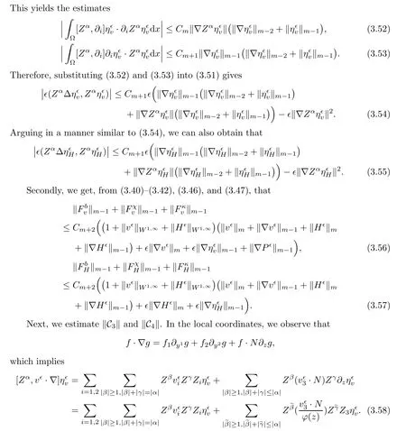
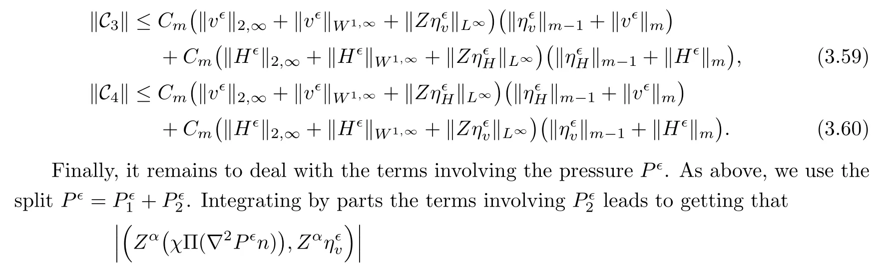

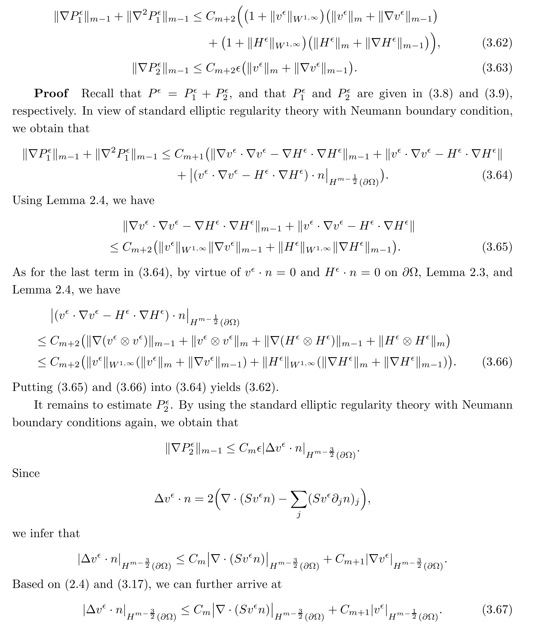
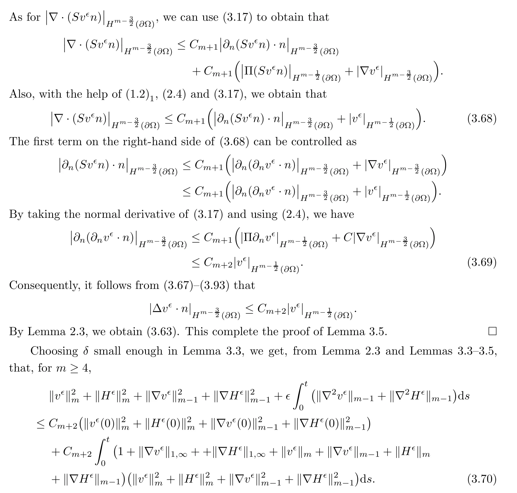
3.3 Pressure Estimates
3.4 L∞estimates


3.5 Proof of Theorem 3.1
3.6 Proof of Theorem 1.1
4 Proof of Theorem 1.3


 Acta Mathematica Scientia(English Series)2021年5期