PM2.5浓度湍流特征和通量获取的实验研究

任燕 李倩惠 张宏升,† 康凌

PM2.5浓度湍流特征和通量获取的实验研究

任燕1,2李倩惠1张宏升1,†康凌3

1.北京大学物理学院大气与海洋科学系, 气候与海‒气实验室, 北京 100871; 2.兰州大学西部生态安全省部共建协同创新中心, 兰州 730000; 3.环境模拟与污染控制国家重点联合实验室, 北京大学环境科学与工程学院, 北京 100871; †通信作者, E-mail: hsdq@pku.edu.cn

利用 PM2.5质量浓度测量仪 E-Sampler 的 1Hz 高频采样功能, 采用涡动相关法, 计算山东省德州大气环境实验站 2018 年 12 月 27 日至 2019 年 1 月 7 日多次污染事件的 PM2.5浓度脉动和湍流通量, 探讨 PM2.5浓度湍流特征。结果表明, 实验观测期间 PM2.5浓度湍流通量均值为 0.026μg/(m2·s); 不同污染过程中 PM2.5浓度湍流通量传输方向不同, 表明不同污染过程的污染源汇属性不同。随着湍流统计特征量(如湍流动能、水平风速标准差、垂直风速标准差、水平风速、动量通量和感热通量)增大, PM2.5湍流垂直通量呈现指数型减小的趋势, 即先急剧减小, 然后随各变量的增长变化不大。随着 PM2.5浓度增大, 其湍流通量绝对值呈现增加趋势, 因此 PM2.5浓度湍流通量的大小与 PM2.5浓度和湍流强弱有关。不稳定条件下, PM2.5浓度归一化标准差与稳定度参数=/遵循−1/3 幂次关系, 即c/*= 6.7(‒ζ)‒1/3; 稳定条件下, 实验结果相对离散。另外, PM2.5浓度脉动方差谱曲线在高频段满足−2/3 幂指数率, PM2.5浓度脉动与垂直速度脉动的协方差谱曲线在高频段满足 −4/3 幂指数率。研究结果表明, 利用 E-Sampler 的 PM2.5浓度 1Hz 高频采样功能可以得到连续且有效的PM2.5浓度湍流通量。

PM2.5浓度湍流通量; 湍流统计特征; 湍流能谱; 污染过程

空气污染严重影响生态环境和人类健康, 并通过气溶胶‒辐射‒云反馈作用影响气候变化。20 世纪 70 年代, 兰州光化学烟雾引起学者的关注; 80—90 年代, 酸雨问题成为大气环境的研究热点; 90 年代后期, 研究者更多地关注改善城市和区域尺度的空气质量[1]。21 世纪以来, 高浓度 PM2.5(空气动力学直径小于等于 2.5μm 的颗粒物)导致霾污染天气现象在京津冀地区频发, 持续时间长, 空间范围广[2‒4]。以 PM2.5为首要污染物霾污染天气现象的发生与污染源排放[5‒6]、气象条件[7‒8]和地形[9]等诸多因素密切相关。霾污染天气发生在大气边界层, 因此大气边界层的结构和特征对污染过程的形成、发展和消散有重要影响[10‒14]。

湍流运动是大气边界层最显著的运动形式, 主导着大气边界层中水‒热和能量的交换与输送[15]。湍流交换决定着污染物能够被传输和扩散的高度以及空间分布。Ren 等[16]发现湍流隔板效应, 并通过实验揭示湍流运动增强或减弱对不同高度 PM2.5浓度变化的影响机制。Wang 等[17]的数值模拟结果表明, 如果强制减弱重污染天气过程中 80%的湍流扩散能力, PM2.5浓度的模拟结果会与观测值更接近, 即修正模式中被高估的湍流扩散作用, 可以有效地改善模式对重污染过程条件下 PM2.5浓度的低估。

毋庸置疑, PM2.5的湍流输送是重霾天气研究中非常重要的内容, 准确地估算 PM2.5的湍流通量不仅有助于精确地计算源排放和污染物输送与沉降, 优化污染排放参数化方案[18‒20], 而且有助于改善霾污染模拟的边界层参数化方案, 提高霾污染天气预报水平[21‒22]。目前, 对 PM2.5湍流输送的研究报道相对较少。与对水汽、二氧化碳等物质的研究不同, 对 PM2.5湍流输送的研究集中在其数浓度[23‒26], 一些研究者也获取了数浓度通量[27‒29]。污染物质量浓度湍流通量能够直接反映其物质情况, 有更广泛的适用性[20,22]。Ren 等[30]将超声风温仪、PM2.5浓度连续测量仪和高频响应消光系数仪构成PM2.5浓度湍流通量测量系统, 其中超声风温仪获取 10 Hz 的垂直风速脉动数据, PM2.5连续测量仪获取PM2.5平均质量浓度数据, 高频响应消光系数仪获取 1 Hz 消光系数数据, 利用大气消光系数与大气气溶胶的关系和规律确定 PM2.5浓度的变化, 采用涡动相关法计算其湍流通量。

鉴于目前没有获取 PM2.5浓度湍流通量的普适性方法, 本文选用文献[30]的结果作为参考, 利用PM2.5质量浓度测量仪 E-Sampler 的 1Hz 高频采样功能, 结合超声风温仪, 基于涡动相关法, 计算和研究 2018 年 12 月 27 日至 2019 年 1 月 7 日德州大气环境实验站PM2.5质量浓度脉动、湍流通量及特征。

1 数据与方法

1.1 实验观测站简介

本研究使用 2018 年 12 月 27 日至 2019 年 1 月 7日山西省德州大气环境实验站的大气湍流和大气环境加强实验观测数据。如图 1 所示, 该实验站位于华北平原(37.15°N, 116.47°E), 周围是较为平坦的农田(图 1(b)), 没有大型的工业排放源。在大气环境实验站安装集成式的三维超声风温仪(IRGASON, Campbell Scientific, Inc., 美国), 架设高度为 2.8m, 传感器朝向正北方向, 采样频率为 10Hz; 架设仪器E-Sampler (Met One, Inc., 美国), 同步进行 PM2.5质量浓度的连续采样, 采样频率可达 1Hz。均采用数据采集器自动采集和记录观测数据, 并实时传输至数据处理中心, 进行数据质控和 30 min 平均。

1.2 数据获取方法与处理

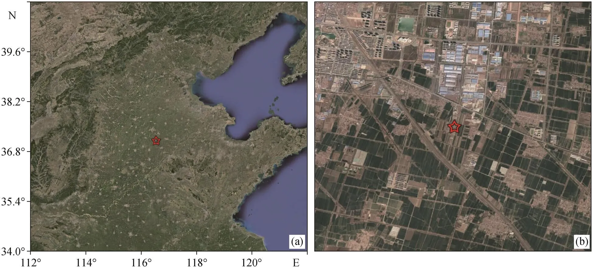
红色五角星代表观测站位置

观测数据的预处理方法如下: 采用 EddyPro 商业软件[31](Advanced 6.2.1, LI-COR Biosciences, Inc.), 对原始湍流数据进行野点剔除[32]、二次坐标变换[33]以及趋势项回归[34]等处理, 并计算各气象要素的湍流统计特征量, 计算时长为 30 min。同时, 对观测数据进行严格的质量控制, 剔除以下数据组: 1)风向与三维超声风温仪传感器的夹角大于±135°的数据组, 即不考虑传感器背后来流方向的数据组(偏南风), 尽量避免仪器支架对流场的影响; 2)不满足梯度输送理论的数据组; 3)明显有错误的数据组。

2 结果和讨论

2.1 PM2.5浓度脉动和湍流垂直通量特征

观测期间包含多次污染天气过程, PM2.5浓度均值为 167μg/m3, 最高可达 676μg/m3; PM2.5浓度脉动值变化范围为±200μg/m3; 污染天气过程的垂直速度脉动数值较小, 变化范围为±2m/s; PM2.5浓度湍流通量变化范围为−1～2μg/(m2·s), 均值为 0.026μg/(m2·s), 与 Ren 等[30]的结果类似, 表明加强实验观测期间德州实验站所在地区整体上为 PM2.5源。如图 2 所示, 污染天气过程个例 1～5 的 PM2.5浓度湍流通量分别为−0.015, −0.030, 0.053, 0.023 和0.078μg/(m2·s)。其中, 个例 1 和 2 的 PM2.5浓度湍流通量方向向下, 表明这两次污染天气过程中德州实验站总体上属于 PM2.5汇, 即以沉降为主; 个例 3～5 的PM2.5浓度湍流通量方向向上, 表明这 3 次污染天气过程中德州实验站总体上属于 PM2.5源, 即以 PM2.5排放为主。可见, 同一地区在不同的污染过程中, 其源汇属性并不是一成不变。

2.2 PM2.5 湍流垂直通量与各湍流变量之间的关系

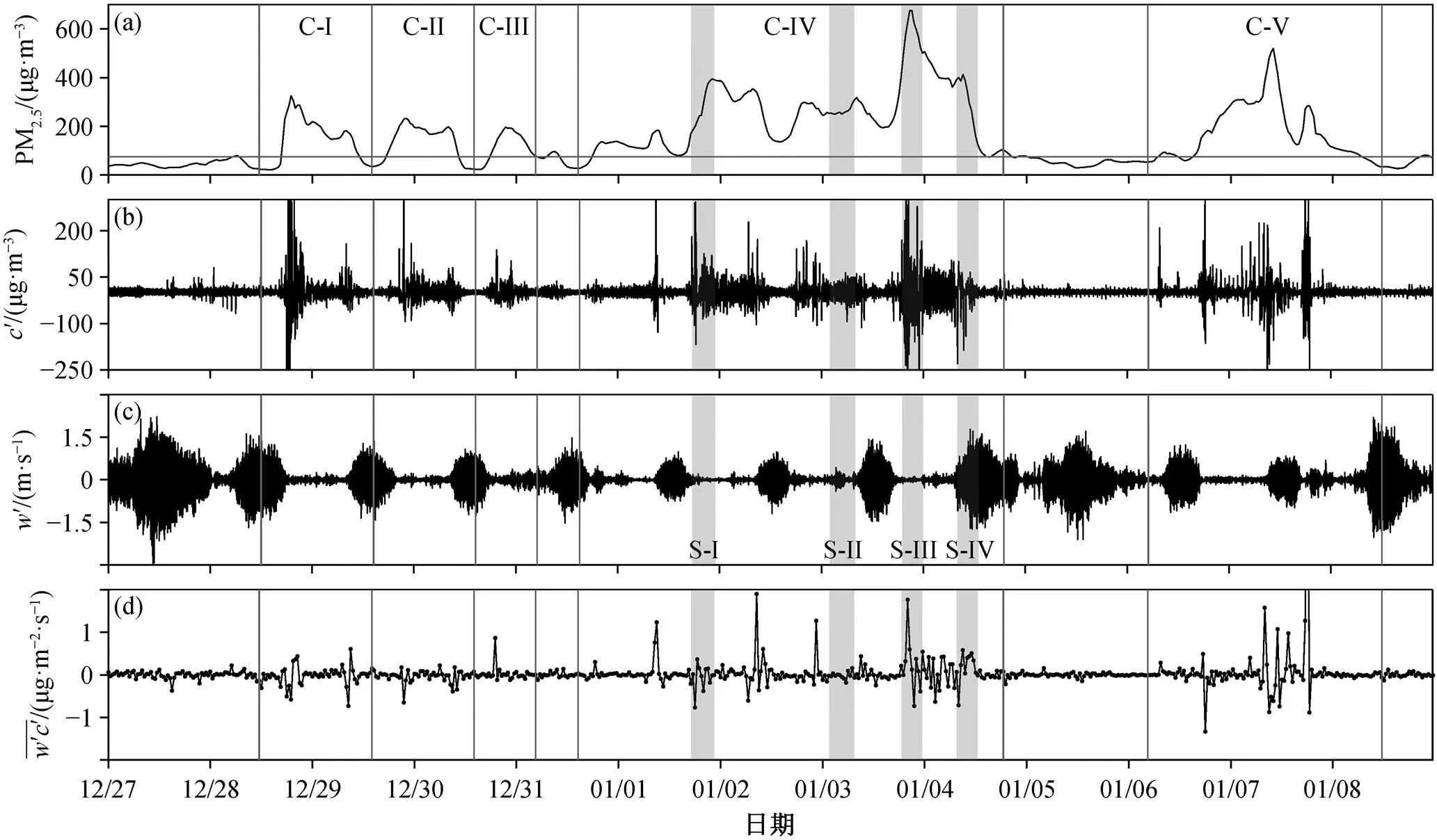
灰色竖线隔开 5 次污染天气过程个例: C-I, C-II, C-III, C-IV, C-V; 灰色阴影区域表示第 4 次污染天气过程的不同阶段: S-I 为污染发展阶段, S-II 为污染维持阶段, S-III 为污染最严重的阶段, S-IV 为污染消散阶段

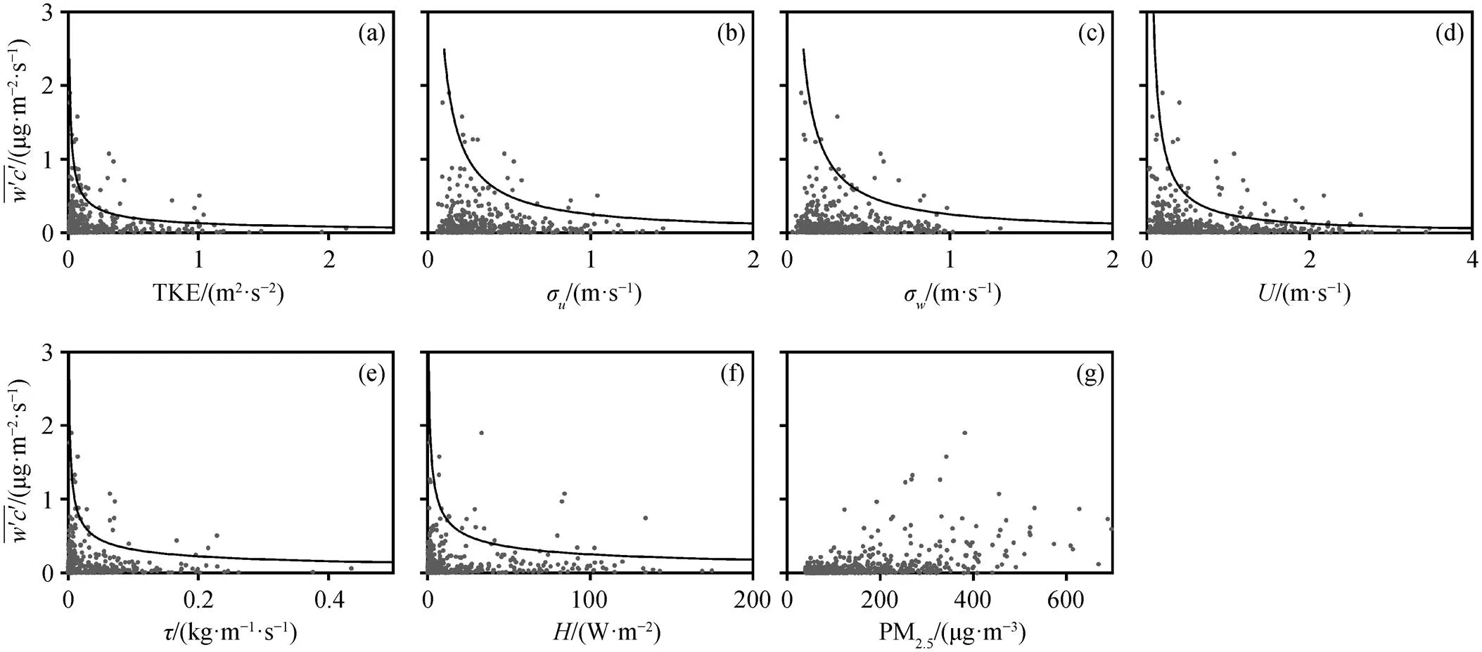
黑色曲线表示湍流垂直通量与其他各湍流变量之间的关系趋势

2.3 PM2.5浓度脉动的湍流特征

近地面层 Monin-Obukhov 相似性理论[35]揭示, 不稳定层结条件下, 三方向风速的归一化标准差与稳定度参数之间存在 1/3 幂次关系, 温度归一化标准差与之间存在−1/3 幂次关系; 近中性层结条件下, 三方向风速的归一化标准差趋近于常数。从图4 可以看到, 近中性条件下, 水平风速归一化标准差/*=2.5(1−2.5ζ)1/3, 略高于文献[36]中平坦下垫面的 2.39±0.03; 温度归一化标准差的系数为 0.8, 略小于文献[37]中美国堪萨斯草原下垫面的 0.95。图 4 显示, 德州大气环境实验观测站测得的风速与温度脉动的统计特征符合经典的相似性关系。

图 4(c1)和(c2)显示, 不稳定条件下, PM2.5浓度归一化标准差与稳定度参数之间的关系也遵循−1/3 幂次关系, 其系数为 6.7, 明显大于温度等标量的归一化标准差的系数, 略小于文献[30]的结果, 原因可能与 PM2.5采样、甄别和处理方式有关; 同时, 也反映 PM2.5浓度湍流特性与温度等标量存在差异。PM2.5浓度的相似性关系与文献[30]相同, 从一个侧面证明本文获取 PM2.5浓度脉动和湍流通量结果的有效性和合理性。

(a1)～(c1) 不稳定条件; (a2)～(c2) 稳定条件

以加强实验观测期间污染过程持续时间最长的个例 4 为例, 根据PM2.5浓度的变化, 将该污染过程分为 4 个阶段: 污染发展阶段(S-I), 污染维持阶段(S-II), 污染最严重的阶段(S-III), 污染消散阶段(S- IV)。图 5 给出 4 个污染阶段水平风速和温度的脉动方差谱, 图 6 给出 4 个污染阶段 PM2.5浓度的脉动方差谱以及 PM2.5浓度脉动与垂直速度脉动的协方差谱。

从图 5(a1)～(a4)可知, 不同污染阶段的水平风速脉动方差谱曲线满足 Kolmogorov 湍流理论[38], 惯性副区满足−2/3 幂次率; 水平风速脉动方差谱的谱峰对应的能谱密度在污染维持阶段(S-II)数值最小; 水平风速脉动方差谱的谱峰对应的能谱密度在污染消散阶段(S-IV)数值最大。原因是, 污染维持阶段的水平风速最小, 污染消散阶段的水平风速最大。温度脉动方差谱曲线呈现类似的规律。从图5(b1)～(b4)可知, 污染发展过程不同阶段的温度脉动方差谱形状相似, 惯性副区满足−2/3 幂次率。

从图 6(a1)～(a4)可知, PM2.5浓度脉动方差谱线形状与水平风速和温度相似, 惯性副区满足−2/3 幂次率。类似地, 图 6(b1)～(b4)中 PM2.5浓度脉动和垂直速度脉动的协方差谱线也呈现与水平风速和温度相似的规律, 惯性副区满足−4/3 幂次率。上述结果表明, PM2.5浓度湍流微观特征符合近地层 Monin-Obukhov 相似性理论[35], 同时验证了 Ren 等[30]的结果。另外, 图 6(a4)、(b1)和(b2)中, PM2.5浓度脉动方差谱以及 PM2.5浓度脉动与垂直速度脉动的协方差谱都在高频位置出现不同程度的噪声, 这一现象表明 PM2.5浓度脉动的高频响应低于风速和温度, 与 E-Sampler 的 PM2.5采样采取抽气的方式有关。

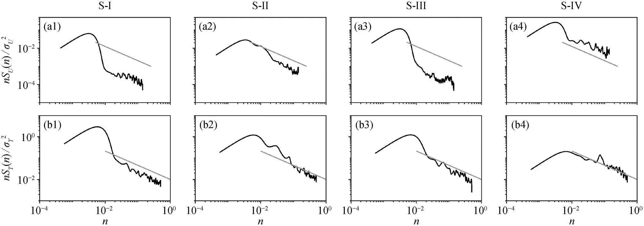
灰色斜线的斜率为−2/3; n表示自然频率

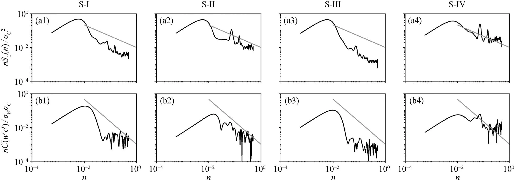
(a1)～(a4)中灰色斜线的斜率为−2/3, (b1)～(b4)中灰色斜线的斜率为−4/3

3 结论

本研究利用 PM2.5质量浓度测量仪 E-Sampler 的1Hz 高频采样功能, 结合超声风温仪, 采用涡动相关法, 计算 PM2.5质量浓度的湍流通量, 讨论 2018年 12 月 27 日至 2019 年 1 月 7 日德州地区 PM2.5浓度的湍流统计特征和微观特征, 证明了获取 PM2.5浓度脉动和湍流通量的可能性和合理性, 得到如下主要结论。

1)利用 PM2.5质量浓度测量仪 E-Sampler 的 1 Hz 高频采样功能, 可以得到连续的 PM2.5浓度脉动及其湍流通量。实验观测期间, 德州大气环境实验站所在地区 PM2.5浓度湍流通量均值为 0.026μg/ (m2·s), 整体上呈现 PM2.5源特征。该期间 5 个污染过程的 PM2.5浓度湍流通量分别为−0.015, −0.030, 0.053, 0.023 和 0.078μg/(m2·s), 表明不同污染天气过程的污染源汇属性有所不同。

2)随湍流统计特征量(如湍流动能、水平风速标准差、垂直风速标准差、水平风速、动量通量和感热通量)增大, PM2.5湍流垂直通量呈指数型减小趋势, 先急剧减小, 然后随各变量的增长变化不大。随着 PM2.5浓度增大, PM2.5浓度湍流通量绝对值呈增加趋势。PM2.5浓度湍流通量的大小与 PM2.5浓度和湍流强弱有关。

3)不稳定条件下, PM2.5浓度归一化标准差/*与稳定度参数的关系遵循−1/3 幂次关系, 即σ/*=6.7(‒)‒1/3。PM2.5浓度脉动方差谱线在惯性副区满足−2/3 幂次率, PM2.5浓度脉动与垂直速度脉动的协方差谱线在惯性副区满足−4/3 幂指次率, 与风速和温度的情况类似, 说明 PM2.5浓度湍流宏观统计特征和微观特征在一定程度上符合近地层 Monin-Obukhov 相似性理论。

[1]Zhu T.Air pollution in China: scientific challenges and policy implications.National Science Review, 2017, 4(6): 800

[2]Fan H, Zhao C, Yang Y.A comprehensive analysis of the spatio-temporal variation of urban air pollution in China during 2014–2018.Atmos Environ, 2020, 220: 117066

[3]Zhang K, Zhao C, Fan H, et al.Toward understanding the differences of PM2.5characteristics among five China urban cities.Asia-Pac J Atmos Sci, 2019, 56: 493–502

[4]Watts J.China: the air pollution capital of the world.Lancet, 2005, 366: 1761–1762

[5]Li M, Liu H, Geng G, et al.Anthropogenic emission inventories in China: a review.National Science Re-view, 2017, 4(6): 834‒866

[6]Zhang Q, Streets D G, Carmichael G R, et al.Asian emissions in 2006 for the NASA INTEX-B mission.Atmos Chem Phys, 2009, 9(14): 5131–5153

[7]Wei W, Zhang H S, Wu B G, et al.Intermittent turbulence contributes to vertical dispersion of PM2.5in the North China plain: cases from Tianjin.Atmos Chem Phys, 2018, 18(17): 12953–12967

[8]Ren Y, Zheng S, Wei W, et al.Characteristics of the turbulent transfer during the heavy haze in winter 2016/17 in Beijing.J Meteor Res, 2018, 32(1): 69–80

[9]Zhang Z, Xu X, Qiao L, et al.Numerical simulations of the effects of regional topography on haze pollu-tion in Beijing.Sci Rep, 2018, 8: 5504

[10]Wei W, Zhang H S, Cai X H, et al.Influence of intermittent turbulence on air pollution in winter 2016/17 over Beijing, China.J Meteor Res, 2020, 34 (1): 176–188

[11]Ren Y, Zhang H, Wei W, et al.Effects of turbulence structure and urbanization on the heavy haze pollution process.Atmos Chem Phys, 2019, 19(2): 1041–1057

[12]Ren Y, Zhang H, Wei W, et al.Comparison of the turbulence structure during light and heavy haze pollution episodes.Atmos Res, 2019, 230: 104645

[13]Ren Y, Zhang H, Wei W, et al.A study on atmospheric turbulence structure and intermittency during heavy haze pollution in the Beijing area.Science China Earth Sciences, 2019, 62(12): 2058–2068

[14]Li Q H, Wu B G, Liu J L, et al.Characteristics of the atmospheric boundary layer and its relation with PM2.5during haze episodes in winter in the North China Plain.Atmos Environ, 2020, 223: 117265

[15]Stull R B.An introduction to boundary layer me-teorology.Dordrecht: Kluwer Academic Publishers, 1988: 9‒19

[16]Ren Y, Zhang H, Zhang X, et al.Turbulence barrier effect during heavy haze pollution events.Sci Total Environ, 2021, 753: 142286

[17]Wang H, Zhang X, Peng Y, et al.The contributions to the explosive growth of PM2.5mass due to aerosols-radiation feedback and further decrease in turbulent diffusion during a red-alert heavy haze in Jing-Jin-Ji in China.Atmos Chem Phys, 2018, 18: 17717–17733

[18]Mårtensson E M, Nilsson E D, Buzorius G, et al.Eddy covariance measurements and parameterisation of traffic related particle emissions in an urban envi-ronment.Atmos Chem Phys, 2006, 6(3): 769–785

[19]Pryor S C, Gallagher M, Sievering H, et al.A review of measurement and modelling results of particle atmosphere–surface exchange.Tellus B: Chemical and Physical Meteorology, 2008, 60(1): 42‒75

[20]Yuan R, Luo T, Sun J, et al.A new method for estimating aerosol mass flux in the urban surface layer using LAS technology.Atmos Meas Tech, 2016, 9(4): 1925‒1937

[21]Jia W, Zhang X.The role of the planetary boundary layer parameterization schemes on the meteorological and aerosol pollution simulations: a review.Atmos Res, 2020, 239: 104890

[22]Ren Y, Zhang H, Zhang X, et al.Temporal and spatial characteristics of turbulent transfer and diffusion coefficient of PM2.5.Sci Total Environ, 782: 146804

[23]Buzorius G, Rannik Ü, Mäkelä J M, et al.Vertical aerosol particle fluxes measured by eddy covariance technique using condensational particle counter.J Aero Sci, 1998, 29(1/2): 157‒171

[24]Dorsey J R, Nemitz E, Gallagher M W, et al.Direct measurements and parameterisation of aerosol flux, concentration and emission velocity above a city.Atmos Environ, 2002, 36(5): 791–800

[25]Martin C L, Longley I D, Dorsey J R, et al.Ultrafine particle fluxes above four major European cities.Atmos Environ, 2009, 43(31): 4714‒4721

[26]Pryor S C, Larsen S E, Sorensen L L, et al.Particle fluxes over forests: analyses of flux methods and functional dependencies.J Geophys Res, 2007, 112 (D7): D07205

[27]Vogt M, Nilsson E D, Ahlm L, et al.The relationship between 0.25–2.5 μm aerosol and CO2emissions over a city.Atmos Chem Phys, 2011, 11(10): 4851–4859

[28]Harrison R M, Dall’Osto M, Beddows D C S, et al.Atmospheric chemistry and physics in the atmosphere of a developed megacity (London): an overview of the REPARTEE experiment and its conclusions.Atmos Chem Phys, 2012, 12(6): 3065–3114

[29]Ripamonti G, Jarvi L, Molgaard B, et al.The effect of local sources on aerosol particle number size distribu-tion, concentrations and fluxes in Helsinki, Finland.Tellus B, 2013, 65: 19786

[30]Ren Y, Zhang H, Wei W, et al.Determining the fluc-tuation of PM2.5mass concentration and its applicabi-lity to Monin–Obukhov similarity.Sci Total Environ, 2020, 710: 136398

[31]LI-COR Biosciences.Eddy covariance processing so-ftware (version 6.2.1) [EB/OL].(2017) [2018‒04‒01].https://www.licor.com/EddyPro

[32]Vickers D and Mahrt L.Quality control and flux sam-pling problems for tower and aircraft data.Journal of Atmospheric and Oceanic Technology, 1997, 14(3): 512‒526

[33]Wilczak J M, Oncley S P, Stage S A.Sonic ane-mometer tilt correction algorithms.Boundary-Layer Meteorology, 2001, 99: 127‒150

[34]Gash J H C, Culf A D.Applying a linear detrend to eddy correlation data in real time.Boundary-Layer Meteorology, 1996, 79: 301‒306

[35]Monin A S, Obukhov A M.Basic laws of turbulent mixing in the atmosphere near the ground.Trudy Geofiz, Inst.AN SSR, 1954, 24: 163‒187

[36]Panofsky H A, Dutton J A.Atmospheric turbulence.New York: John Wiley & Sons, 1984: 156‒173

[37]Wyngaard J C, Coté O R, Izumi Y.Local free convection, similarity, and the budgets of shear stress and heat flux.Journal of Atmospheric Sciences, 1971, 28(7): 1171‒1182

[38]Kolmogorov A N.The local structure of turbulence in incompressible viscous fluid for very large Reynolds numbers.Cr Acad Sci URSS, 1941, 30: 301‒305

Experimental Study on the Turbulence Characteristics and Flux Acquisition of PM2.5

REN Yan1,2, LI Qianhui1, ZHANG Hongsheng1,†, KANG Ling3

1.Laboratory for Climate and Oceanic-Atmosphere Studies, Department of Atmospheric and Oceanic Sciences, School of Physics, Peking University, Beijing 100871; 2.Collaborative Innovation Center for West Ecological Safety, Lanzhou University, Lanzhou 730000; 3.State Key Joint Laboratory of Environmental Simulation and Pollution Control, College of Environmental Sciences and Engineering, Peking University, Beijing 100871; † Corresponding author, E-mail: hsdq@pku.edu.cn

The authors use the high-frequency sampling function of the fine particle mass concentration measurement instrument E-Sampler and the eddy covariance method to calculate PM2.5concentration fluctuation and turbulent flux of the multiple pollution events of the Dezhou city atmospheric environment experimental station in Shandong Province from December 27, 2018 to January 7, 2019, and the turbulence characteristics of PM2.5concentration are discussed.The results show that the mean value of the turbulent flux of PM2.5concentration during the observation period is 0.026 μg/(m2·s).The transmission direction of the turbulent flux of PM2.5concentration in different pollution processes is different, indicating that the sink or source property is not static.With the increase of turbulence statistical characteristic quantities (such as turbulent kinetic energy, standard deviation of horizontal wind speed, standard deviation of vertical wind speed, horizontal wind speed, momentum flux and sensible heat flux), the vertical flux of PM2.5decreases exponentially, namely, it decreases sharply, and then changes little with the increase of each variable.With the increase of the concentration of PM2.5, the absolute value of the turbulent flux of PM2.5shows an increasing trend.The turbulent vertical flux of PM2.5concentration is related to the PM2.5concentration and the intensity of turbulence.The normalized standard deviation of PM2.5concentration and the stability parameter=/follow the −1/3 power relationship under unstable conditions, that isc/*=6.7(−ζ)−1/3.Under stable conditions, the experimental results are relatively discrete.In addition, the variance spectrum curve of PM2.5concentration satisfies the −2/3 power exponential rate in the high frequency range, and the covariance spectrum curve of the PM2.5concentration and the vertical wind speed satisfies the −4/3 power exponential rate in the high frequency band.The result shows that 1Hz high-frequency sampling function of E-Sampler can obtain continuous and effective turbulent flux of PM2.5concentration.

turbulent flux of PM2.5concentration; turbulence statistics; turbulence energy spectrum; pollution process

10.13209/j.0479-8023.2021.082

2020–11–22;

2021–01–20

国家重点研发计划(2017YFC0209904, 2017YFC0209600)、国家自然科学基金(41705003, 41544216)和新疆维吾尔自治区高层次(柔性)人才引进项目(2018)资助