HYBRID REGULARIZED CONE-BEAM RECONSTRUCTION FOR AXIALLY SYMMETRIC OBJECT TOMOGRAPHY*

Xinge LI (李兴娥) Suhua WEI (魏素花) Haibo XU (许海波)

Institute of Applied Physics and Computational Mathematics，Beijing 100094，China E-mail:li_xinge@iapcm.ac.cn;wei_suhua@iapcm.ac.cn;xu_haibo@iapcm.ac.cn

Chong CHEN (陈冲)†

LSEC，ICMSEC，Academy of Mathematics and Systems Science，CAS，Beijing 100190，China E-mail:chench@lsec.cc.ac.cn

Abstract In this paper，we consider 3D tomographic reconstruction for axially symmetric objects from a single radiograph formed by cone-beam X-rays.All contemporary density reconstruction methods in high-energy X-ray radiography are based on the assumption that the cone beam can be treated as fan beams located at parallel planes perpendicular to the symmetric axis，so that the density of the whole object can be recovered layer by layer.Considering the relationship between different layers，we undertake the cone-beam global reconstruction to solve the ambiguity effect at the material interfaces of the reconstruction results.In view of the anisotropy of classical discrete total variations，a new discretization of total variation which yields sharp edges and has better isotropy is introduced in our reconstruction model.Furthermore，considering that the object density consists of continually changing parts and jumps，a high-order regularization term is introduced.The final hybrid regularization model is solved using the alternating proximal gradient method，which was recently applied in image processing.Density reconstruction results are presented for simulated radiographs，which shows that the proposed method has led to an improvement in terms of the preservation of edge location.

Key words high-energy X-ray radiography;cone-beam global reconstruction;inverse problem;total variation;alternating proximal gradient method

1 Introduction

Computerized tomography is a technique that inverts“projection data sets”to form an estimate of density at each point inside an object.The mathematical basis of the method is the reconstruction of a three-dimensional function from a set of line integrals.The earliest treatment of this problem in two dimensions was given by Radon in 1917[1].Nowadays，many strategies are available，and most of them have been widely used in medical imaging diagnosis and industrial nondestructive detection.

In high-energy X-ray radiography，two-dimensional detectors are used for image acquisition.In these scenarios，the object size is very small，the cone-beam geometry has a relatively small divergent angle，and fan-beam reconstruction is the most popular reconstruction method.To get three-dimensional images，a series of two-dimensional cross-sectional images of an object are made from one-dimensional projections and“stacked”on top of each other[2，3].This method does not consider the relationship between different cross sections，so the blur cannot be eliminated and the interface positions are not correct.Moreover，when the divergent angle of the cone-beam geometry gets bigger，this layered fan-beam approximation no longer works.

To overcome the disadvantages of fan-beam reconstruction，we concentrate on cone-beam reconstruction using multiple two-dimensional projection image at one time.Over the years，a number of researchers have proposed various methods for cone-beam reconstruction.Existing cone-beam algorithms can be categorized into two broad classes:analytic and algebraic[4-6].Among the various approaches，Feldkamp’s heuristically derived algorithm[7]is the most efficient and most suitable to parallel processing[8].It is an extension of the conventional equispatial fan-beam reconstruction algorithm，where two-dimensional projection data from different angles are filtered and backprojected to voxels along projection beams.The final value of each voxel is the sum of contributions from all tilted fan-beams passing through the voxel.The algebraic approach consists of constructing a set of linear equations whose unknowns are elements of the object cross section，and then solving these equations with iterative methods[9-11].The coefficient matrix of this system of linear equations is often known as the imaging matrix，or the forward projection matrix.The mesh generation of the object determines the construction of the projection matrix，and we adopt an efficient calculation method similar to that used in[12].Considering the restrictions of the analytic and algebraic methods on data acquisition and quality，we employ the latest variational method for density reconstruction in high-energy X-ray radiography using measurements with complex engineering factors involved.

Variational methods can incorporate into the solution some types of a priori information about the density image to be reconstructed.In an influential paper，Rudin，Osher，and Fatemi[13]suggested using the total variation (TV) regularization functional to smooth images.As about the same time，Bouman and Sauer[14]proposed a discrete version of the TV in the context of tomography.TV minimization has since found a use in a wide range of problems to recover sharp images by preserving strong discontinuities，while removing noise and other artifacts[15-17].In the continuous setting，the TV is simply the L1norm of the gradient amplitude，but for discrete images，it is a nontrivial task to properly define the gradient using finite differences.

Most algorithms approximate the continuous TV by a sum of the L2norm of a discrete finite difference estimate of the image gradient，called an isotropic scheme，denoted as

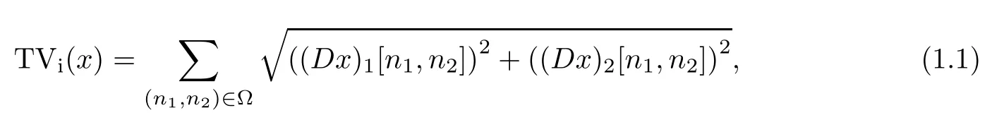
where

for every (n1，n2)∈Ω，with Neumann boundary conditions，and x:Ω→R being a discrete gray-level image defined on the finite domain Ω⊂Z2.This so-called isotropic TV is actually far from being isotropic，but it performs reasonably well in practice.In some situations，an anisotropic scheme (L1norm) may be used[18，19]，leading to the anisotropic discrete TV

The minimization of this favors horizontal and vertical structures，because oblique structures make for a larger TVavalue.New discrete schemes have recently been proposed[20-23]to improve the isotropy of the discrete TV.In particular，the new definition in[21]is based on the idea of associating an image with a gradient field on a twice finer grid in a bilinear way.The TV of the image is then simply the L1norm of this gradient field amplitude.This corrects some drawbacks of the classical definition and yields sharper edges and structures.In this paper，we apply this new discretization to the total variation regularization of cone-beam reconstruction.

The TV minimization preserves edges well but can cause staircase artifacts in flat regions.Staircase solutions fail to satisfy the eyes and they can develop false edges that do not exist in the true image.In order to overcome these model-dependent deficiencies，there is growing interest in the idea of replacing the TV by the high-order TV.There are two classes of second-order regularization methods.The first class combines a second-order regularizer with the TV norm.For example，a novel and effective model that combines the TV with the Laplacian regularizer was presented for image reconstruction in[3].A technique in[24，25]，combining the TV filter with a fourth-order PDE filter，was proposed to preserve edges and at the same time avoid the staircase effect in smooth regions for noise removal.In[26，27]，the authors considered a high-order model involving convex functions of the TV and the TV of the first derivatives for image restoration.Chan，et al.，in[28]，proposed a second-order model to substantially reduce the staircase effect，while preserving sharp jump discontinuities.The second class employs a second-order regularizer in a standalone way.For example，in[29-32]，the authors considered a fourth-order partial differential equations (PDE) model for noise removal.Benning analyzed the capabilities and limitations of three different higher-order TV models and improved their reconstructions in quality by introducing Bregman iterations in[33].Hessian-based norm regularization methods were effectively used in[34]for image restoration and in applications such as biomedical imaging.

In this paper，we focus on cone-beam global reconstruction based on hybrid regularization.The main contributions of this paper are as follows:

1.A special discretization scheme for the scanning object is proposed to fully utilize its axially symmetric property;this helps to constrain the reconstruction space and simplify the computations.

2.A new discrete approximation to the isotropic TV is adopted for better preservation of tilt edges.

3.A second-order regularization term is introduced in the reconstruction of piecewise smooth images.

The rest of the paper is organized as follows:Section 2 briefly reviews the new TV discretization proposed in[21].In Section 3，the mathematical model of density reconstruction is described in detail.In Section 4，we solve the hybrid regularization model with the alternating proximal gradient method (APGM).Numerical experiments comparing the results of the new model and other possible regularization techniques are presented in Section 5.Finally，a summary and outlook are contained in Section 6.

2 Review of the New TV Discretization

It is well known that in the continuous domain，the TV of a function s can be defined by duality as

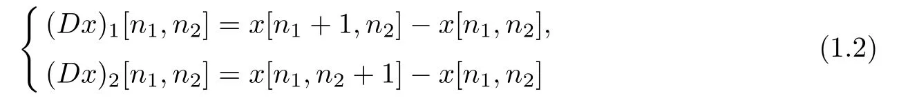
Note that for ease of implementation，it is convenient to have all images of the same size，N1×N2，indexed by (n1，n2)∈Ω.First，the so-called isotropic TV of an image x can be defined by duality as

The scalar dual variables u1[n1，n2]and u2[n1，n2]，like the finite differences (Dx)1[n1，n2]and (Dx)2[n1，n2]，can be viewed as being located at the points (n1+，n2) and (n1，n2+)，respectively.Therefore，the anisotropy of the isotropic TV can be explained by the fact that these variables，which are combined in the constraint|u[n1，n2]|≤1，are located at different positions.To correct this half-pixel shift，bilinear interpolation is utilized and the discrete TV is defined in the dual domain as

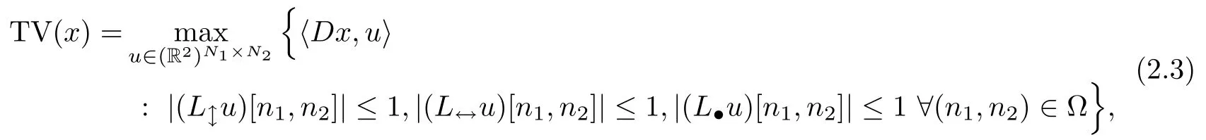
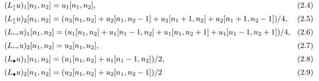
where the three operators L↕，L↔，L·interpolate bilinearly the image pair u=(u1，u2) on the grids，(n1，n2)，for (n1，n2)∈Ω，respectively (see Figure 1).That is，

Figure 1 The locations of intensity values for each pixel are shown by·circles，the locations of (Dx)1(n1，n2)，u1(n1，n2) are shown by↕，and the locations of (Dx)2(n1，n2)，u2(n1，n2) are shown by↔.

for every (n1，n2)∈Ω，replacing the dummy values u1[N1，n2]，u2[n1，N2]，(L↕u)1[N1，n2]，(L↕u)2[N1，n2]，(L↔u)1[n1，N2]，(L↔u)2[n1，N2]by zero.Thus，the continuous definition (2.1)，where the dual variable is bounded everywhere，is mimicked by imposing that it is bounded on a grid three times more dense than the pixel grid.

In the frame of the Fenchel-Rockafellar duality[35]，the discrete TV can be defined as the optimal value of an equivalent optimization problem，expressed in terms of the gradient field of the image.That is，

where·*denotes the adjoint operator.Let the vector field v be the concatenation of the three vector fields v↕，v↔，and v·.Let the L1，1，2norm of v be the sum of the L1，2norm of its three components v↕，v↔，and v·，where the L1，2norm is the sum over all pixels of the L2norm.Set L*v=.Then (2.10) can be rewritten as

with zero boundary conditions.Thus，the quantityis the sum of the vertical part of the elements of the vector field v falling into the square[n1，n1+1]×，weighted by 1/2 if they are on an edge of the square，and by 1/4 if they are at one of its corners.Similarly，is the sum of the horizontal part of the elements of v falling into the square×[n2，n2+1].

Given an image x，let v↕，v↔and v·denote the vector fields solution to (2.10)(or any solution if it is not unique).Let v denote the vector field，which is the concatenation of v↕，v↔and v·.Then，for every (n1，n2)∈Ω，the elements v↕[n1，n2]，v↔[n1，n2]，v·[n1，n2]are vectors of R2located at the positions，(n1，n2)，respectively.Then v is called the gradient field of x.Thus，the discrete TV is the L1，1，2norm of the gradient field v associated to the image x，is the solution to (2.10)，and is defined on a grid three times more dense than the one of x.The mapping from x to its gradient field v is nonlinear and implicit:given x，one has to solve the optimization problem (2.10) to obtain its gradient field and the value TV (x).

3 Mathematical Model of Density Reconstruction

In this section，we introduce the mathematical model of density reconstruction.For the sake of presentation，we are going to use the same notation for scalars and vectors.In our experimental setting，a radially symmetric object with radius R and height H is situated so that its center-layer lies in the ξη-plane and its axis of symmetry coincides with the ζ-axis (see Figure 2).Only a single radiograph is taken with a radiographic axis perpendicular to the symmetric axis of the object.The transmitted radiation is measured by a detector lying on a plane ξ=ξ0.Images captured by X-ray imaging systems are direct measures of the optical density.The measured optical density can be converted to areal density，which combines both the volumetric densities of the materials and their thicknesses.

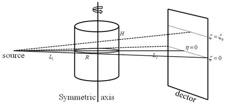
Figure 2 Illustration of the single radiograph imaging system for axially symmetric objects

The areal density b，sometimes referred to simply as the projection data，is related to the object density ρ by the line integral along the X-ray track

where μρare the material’s mass attenuation coefficients，and μl=μρρ are the material’s linear attenuation coefficients.In order to reconstruct the density distribution of the object，we need to discretize this integral.First，a three-dimensional concentric ring grid is generated for the axisymmetric object;that is，slices of equal thickness Δh along the axis of symmetry (see Figure 3(a))，and concentric rings centered on the axis of symmetry with equal radius Δr perpendicular to the axis of symmetry (see Figure 3(b)).On the basis of this grid，the forward projection matrix A defined by line integrals can be obtained;the nonzero elements of this are lengths of adjacent intersections between X-ray and concentric ring grid.Hence (3.1) is then discretized as

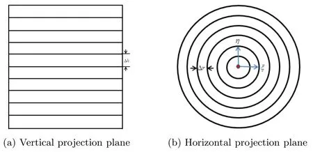
Figure 3 Projection of the radially symmetric object

where A∈Rm×n;b∈Rmare the areal density values;the unknown x∈Rnhere are actually the linear attenuation coefficients，and the density values to be reconstructed can be obtained by dividing the linear attenuation coefficients by the material’s mass attenuation coefficients.Here，m is a fixed number determined by the projection data，and n is independently chosen according to the discretization of ρ.

Noting that our object partition mesh is different from the traditional voxel partition，we describe the construction method of the projection matrix in detail.Specifically，we use Xray tracing to calculate the matrix A with an arbitrary source point O (ξO，ηO，ζO)，a detected point R (ξR，ηR，ζR)，and its projecting point R′(ξR，ηR，ζO) at a horizontal plane at ζ=ζO(see Figure 4).The X-rayintersects with the object and its projection isin plane ζ=ζO.At this plane，the X-ray intersects with the concentric circles of the gridded object and forms n+1 points of intersection.In Figure 4(a) the distance from the source point O to the intersecting point is

where O*is the center point of the object，is the length of the vector，ψ is the angle between vectors，and r is the radial coordinate of the intersecting point.Using (3.3) we obtain ordered distances of the.Then projectingback to，the lengths of the X-rayintersections with the object are obtained as/cosφ，where φ is the angle between the vectors.

Then we calculate the distance from the source point O to the intersection of the X-ray and the gridded object at the vertical slices on Figure 4(b).Because the q-th slice position is at plane ζ=ζq，the distanceis

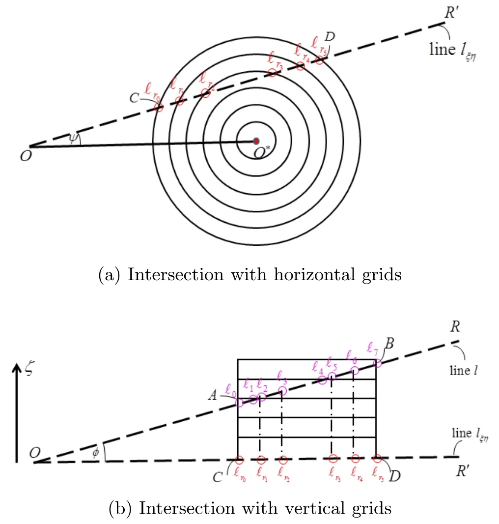
Figure 4 The intersection of the X-ray and gridded object

where ϑ is the cosine of the angle between the vectorand the ζ-axis.Now，we put all the distances into a set

Sorting in ascending order gives the set C′={ℓ0，ℓ1，···，，···，ℓn+m+1}，where n′is the index of the intersecting point.Let i and j denote the indexes of the detector pixel and the object voxel，respectively.If the segmentlies in the j-th voxel，the projection matrix element aijthen follows as

Considering the degradations that may occur during the imaging process，we deal with the general observation model given by

where ε∈Rmdenotes the unknown noise，and K∈Rm×mpresents the blurring that may be produced in the process of radiographing，including the source blur and the detector blur.

Since the inverse problem (3.6) is ill-posed，researchers have proposed a number of regularization methods[3，36-39].All of these methods can be formulated as solving a minimization problem of the form

where R (x) is a regularization functional，and λ＞0 is the regularization parameter.Since the density values are nonnegative and gradually varied in one material，but have sharp jumps between different materials，that is，the unknown x’s are nonnegative and piecewise smooth，we introduce the nonnegative constraint，the TV norm and the Laplace term into the minimization problem (3.7).Then we derive the hybrid regularized density reconstruction model

where Δ is the discrete Laplacian operator，and λ，μ＞0 are regularization constants that need to be properly chosen.

4 Algorithm for the Hybrid Regularization Model

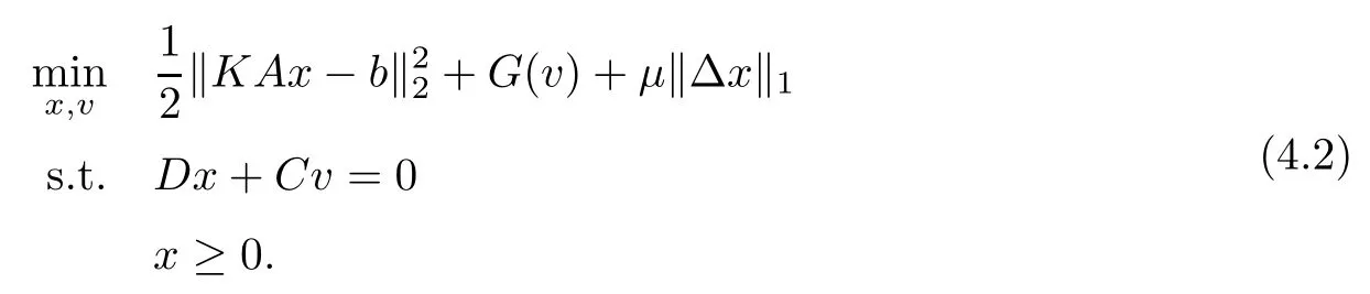
In this section，we discuss the algorithm for solving the hybrid regularization model (3.8).This can be rewritten as

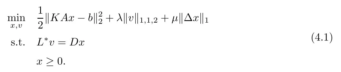
Thus，we have to find not only the image，but also its gradient field，minimizing a separable function under a linear coupling constraint.Let us introduce the function G (v)=λ‖v‖1，1，2and the linear operator C=-L*，so that we can put (4.1) into the standard form

First，we consider the more general problem

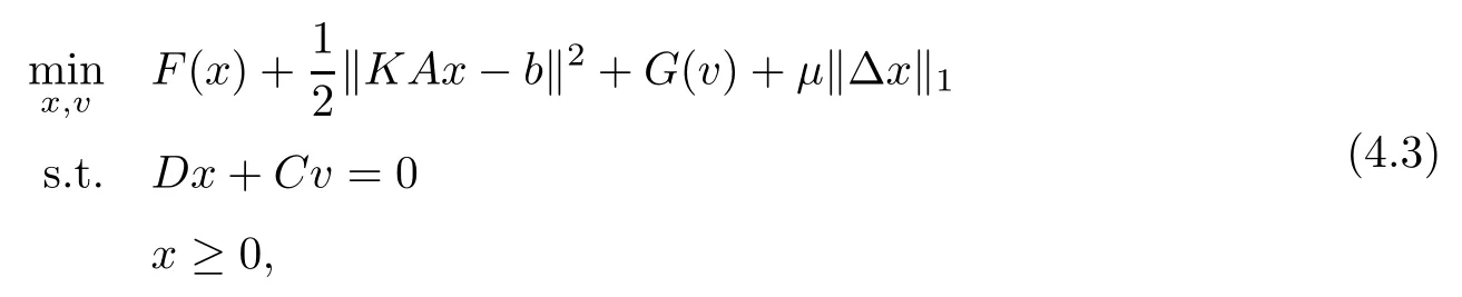
where F is a convex，proper，lower semicontinuous function[35].The constraint x≥0 can be put into the objective function by using an indicator function:

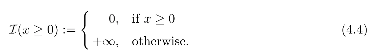
This leads to the following equivalent reformulation of (4.3):

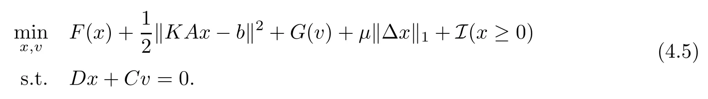
Recently，an alternating proximal gradient method (APGM) for solving the convex optimization problem (4.5) was proposed[40].APGM is based on the framework of the alternating direction method of multipliers (ADMM)，but all the subproblems in APGM are easy to solve.In fact，when APGM is applied to solve (4.5)，two subproblems of APGM correspond to the proximal mappings of F and G，respectively.Thus all the problems that are difficult to solve by ADMM can be solved easily by APGM.

Note that the proximal mapping of F (x)+μ‖Δx‖1+I (x≥0) is not easy to compute，so we need to further split the three functions.To this end，we introduce two new variables，w and z，and rewrite (4.5) as

Noticing that in (4.6) there are four blocks of variables，x，v，w and z，we can group v，w and z into one big block，and rewrite (4.6) in the form

where X=[x]，Y=[v;w;z]，R=[D;Δ;I]，S=diag (C，-I，-I)，F′(X)=F (x)+‖KAxb‖2，and G′(Y)=G (v)+μ‖w‖1+I (z≥0).By attaching a Lagrange multiplier vector Q=[q1;q2;q3]to the linear constraints RX+SY=0，the augmented Lagrangian function Lγ(x，v，w，z;q1，q2，q3) is defined as

where γ＞0 is a penalty parameter.Then the APGM for solving (4.6) can be described as

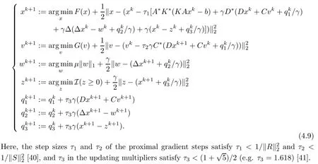
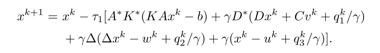
We now show how to solve the four subproblems in (4.9).For our reconstruction model，F (x)=0，so the first subproblem in (4.9) corresponds to

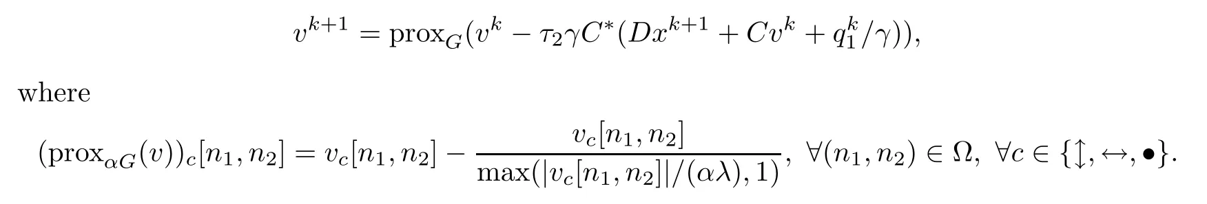
The second subproblem in (4.9) is given by the proximity operator of G

The third subproblem in (4.9) has a closed-form solution which is given by the soft thresholding

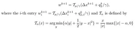
for x∈R，α＞0(see[42]).The fourth subproblem in (4.9) corresponds to projecting the vector xk+1+onto the nonnegative orthant and this can be done by zk+1=max{xk+1+，0}，where the max function is componentwise.

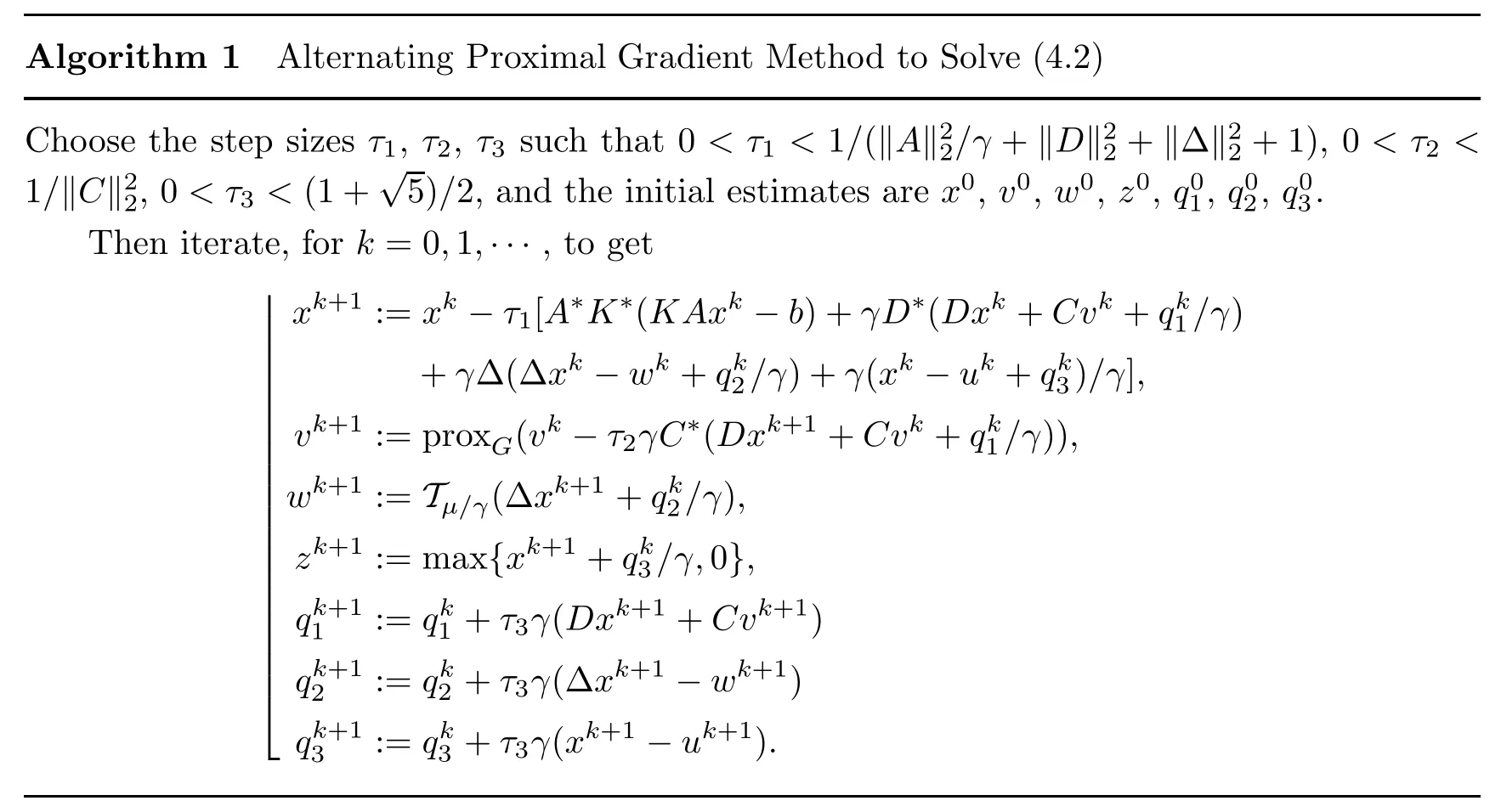
The convergence of Algorithm 1 can be monitored using primal and dual“residuals”，which are defined as rk=RXk+SYkand dk=γRTS (Yk-Yk-1) respectively[43]，both of which approach zero as the iterates become more accurate.The iteration is generally stopped when

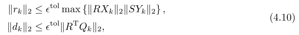
where∈tol＞0 is the stopping tolerance，and a reasonable value might be∈tol=10-3or 10-4，depending on the application.

It is well known that the correct choice of the penalty parameter plays a vital role in obtaining good convergence.With the goal of improving the convergence in practice，as well as making performance less dependent on the initial choice of the penalty parameter，we choose to use different penalty parameters γkfor each iteration.A simple scheme that often works well is

where β＞1，τincr＞1 and τdecr＞1 are parameters[43].Typical choices might be β=10 and τincr=τdecr=2.This penalty parameter update is based on the observation that increasing γkstrengthens the penalty term，yielding smaller primal residuals but larger dual ones;conversely，decreasing γkleads to larger primal and smaller dual residuals.As both residuals must be small at convergence，it makes sense to“balance”them，i.e.，tune γkto keep both residual norms within a factor of β of one another.

5 Numerical Results

In this section，we show the numerical results of the proposed model on the tomographic reconstruction for general cylindrically symmetric objects (3D) from a single radiograph.All the results were generated using a computer with Intel core 2.83GHz CPU，4 threads，and 8GB of memory.The radiograph is taken by cone-beam X-rays.In our imaging system (see Figure 2)，R，H，L1，L2are taken to be 7cm，14cm，350cm and 105cm，respectively.We take 113 partitions for the radius R，227 partitions for the height H，and 2252measuring points for b.The simulated radiograph is contaminated by Gaussian white noise.The blur in the imaging process is treated as Gaussian，and the blurring matrix K is substituted by the Gaussian matrix.

To evaluate of the reconstruction quality，we can have an“eyeball”impression.Since in high-energy X-ray radiography we focus more on the recovery of material interfaces，the Canny edge detection algorithm[44]is used to show the distributions of boundaries in the reconstruction results so as to judge and select a satisfactory reconstruction.The Canny operator takes as input a gray scale image，and produces as output an image showing the positions of tracked intensity discontinuities.In this paper，we use the MATLAB command

edge (x，’canny’)

to generate the distributions of edges in all reconstruction results.We do not specify sensitivity thresholds for the Canny method，and edge chooses low and high values automatically.

5.1 Test for piecewise constant object

To observe the effect of different discretizations of total variation on reconstruction results，we set μ=0.0 in the model (3.8)，and reconstructed the French Test Object (FTO)(see Figure 5(a)) from the noisy radiography shown in Figure 5(b).The noise variance here is taken to be 1.5%of the maximum noiseless projection data.Figure 5(c-h) show the reconstruction results of the TV regularization technique based on discretizations (1.1)，(1.3) and (2.11)，and their corresponding Canny edge distributions.We set λ=0.4 for the models based on these three TV discretizations.Note that the reconstruction results are shown with pseudo color images，which can better highlight the reconstruction effect at the material interfaces.The actual boundaries have been marked with colored lines in Figure 5(a).Compared with the true density pro file (a)，we find that the solution of the new TV model (g) has the best reconstruction effect，followed by the isotropic TV model (e) and the anisotropic TV model (c).It should be pointed out that there are some pseudo-edges in both (d) and (f)，and the boundaries in (h) exactly match the real boundaries in (a).It is not difficult to find that the new discretization has the best reconstruction effect at the material interfaces，especially at the inclined boundary (non-horizontal or vertical boundary).

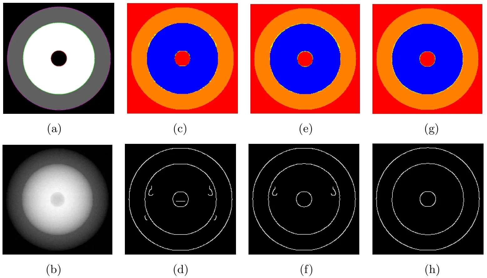
Figure 5 3D tomographic reconstructions and the corresponding Canny edge distributions for the FTO.(a) True densit profile;(b) noisy projection data;(c，d) anisotropic TV model;(e，f) isotropic TV model;(g，h) new TV model.

5.2 Test for piecewise smooth object

We now analyze the advantages of hybrid regularization in restoring density distribution with piecewise smoothness.For this purpose，we simulate two spherical objects whose density cross sections passing through the axis of symmetry are shown in Figure 6(a) and Figure 7(a)，and reconstruct them using the anisotropic TV model，the isotropic TV model，the new TV model and the hybrid regularization model，respectively.The density function in Figure 6(a) is a piecewise smooth function of radius，which is called“DISK”.Figure 7(a) is a simulated face image whose density function has more sharp edges than Figure 6(a)，which is called“FACE”.The true edges are marked with colored lines in Figure 6(a) and Figure 7(a).Their radiographs are shown in Figure 6(b) and Figure 7(b)，which are corrupted by Gaussian noise with the noise variance taken to be 1.5%of the maximum of noiseless projection data.For these two tests，we choose λ=0.4，μ=0.0 for the single TV models，and λ=0.4，μ=0.2 for the hybrid regularization model.The reconstruction results are shown in Figure 6(c，f，i，l) and Figure 7(c，f，i，l)，the zoom-in views of the regions located in the red frames are shown in Figure 6(d，g，j，m) and Figure 7(d，g，j，m)，and the Canny edge distributions are shown in Figure 6(e，h，k，n) and Figure 7(e，h，k，n).It is easy to see that the solutions of the single TV models have an obvious staircase effect，which leads to many pseudo-edges in their edge distributions.Moreover，the solution of the hybrid regularization model is in better agreement with the true value，which also verifies the advantages of the proposed method.

6 Conclusion

In this paper，we have proposed a hybrid regularized density reconstruction model with nonnegative constraints based on a new discretization of total variation，and solved it by the alternating proximal gradient algorithm，in which all the subproblems are easy to solve compared with ADMM.Numerical results have shown that the new discretization of total variation is more isotropic and has a better reconstruction effect at the material interfaces.Furthermore，the hybrid regularization is more advantageous than the total variational regularization in the reconstruction of piecewise smooth images.

The new discretization of total variation achieves better behavior on oblique structures.Since there is no conflict between the anisotropic，isotropic and new discretization schemes，these ideas can work together and further improve the edge preserving property of TV regularization.In the future，we will explore the adaptive formulation for the discrete total variation based on the intrinsic geometrical properties of an image，such as the edge orientation.We will also consider edge detection based on the gradient amplitude computed with the new definition of the gradient field of an image.