Free-boundary plasma equilibria with toroidal plasma flows

Wenjin CHEN(陈文锦),Zhiwei MA (马志为),*,Haowei ZHANG (张豪伟),Wei ZHANG (张威)and Longwen YAN (严龙文)

1 Institute for Fusion Theory and Simulation,Zhejiang University,Hangzhou 310027,People’s Republic of China

2 Southwestern Institute of Physics, Chengdu 610225, People’s Republic of China

Abstract Magnetohydrodynamic equilibrium schemes with toroidal plasma flows and scrape-off layer are developed for the ‘divertor-type’ and ‘limiter-type’ free boundaries in the tokamak cylindrical coordinate.With a toroidal plasma flow, the flux functions are considerably different under the isentropic and isothermal assumptions.The effects of the toroidal flow on the magnetic axis shift are investigated.In a high beta plasma,the magnetic shifts due to the toroidal flow are almost the same for both the isentropic and isothermal cases and are about 0.04a0 (a0 is the minor radius)for M0=0.2(the toroidal Alfvén Mach number on the magnetic axis).In addition, the X-point is slightly shifted upward by 0.0125a0.But the magnetic axis and the X-point shift due to the toroidal flow may be neglected because M0 is usually less than 0.05 in a real tokamak.The effects of the toroidal flow on the plasma parameters are also investigated.The high toroidal flow shifts the plasma outward due to the centrifugal effect.Temperature profiles are noticeable different because the plasma temperature is a flux function in the isothermal case.

Keywords: tokamak plasma, plasma flow, equilibria

1.Introduction

In the past decades,plasma flows have been observed in almost all tokamaks.It can be either spontaneous [1] or driven by neutral beam injection[2]or radio frequency wave heating[3].Some advanced diagnostic technologies have been developed to measure plasma flow, such as charge exchange recombination spectroscopy [4], imaging x-ray crystal spectrometer [5],Doppler coherence imaging spectroscopy[6, 7]and Langmuir probe.With diagnostic developments, the effects of plasma flows have been investigated intensively.It is found that either toroidal or poloidal plasma flows could suppress macroscopic instabilities, such as(double)tearing mode[8,9] and resistive wall mode [10], and then largely improve both energy and momentum confinement[11,12].The penetration properties of the n=1 resonant magnetic perturbation are also strongly correlated with toroidal flows [13, 14].

For static and ideal plasma, the equilibrium with the axisymmetric assumption can be obtained by solving the well-known Grad–Shafranov (GS) equation that is the nonlinear partial differential equation for poloidal magnetic flux ψ.There are two free flux functions, pressure p(ψ) and poloidal current function F(ψ), in the GS equation.Several famous static equilibrium codes,such as CHEASE[15],EFIT[16,17],HELENA[18],NOVA q-solver[19]and so on,were developed to solve the GS equation successfully.In order to consider a toroidal plasma flow in the equilibrium, the GS equation has to be generalized.Several codes,such as FLOW[20], ATEC [21], CLIO [22], FINESSE [23], and M3D equilibrium solver[24],have also been developed to solve the generalized GS (GGS) equation [25, 26], which is able to obtain two types of the equilibria: isentropic equilibrium and isothermal equilibrium.In the isentropic equilibrium, it is assumed that the entropy S=S(ψ) is constant on magnetic surfaces, which considers the isotropic plasma and holds for isentropic flowB·∇S(ψ )=0.In the isothermal equilibrium, the plasma temperature is assumed to be a surface quantity T=T(ψ)because of the large heat conductivity along the magnetic field line within a flux surface, which implies isothermal flowB·∇T(ψ)=0.In this paper, a detailed comparison between these two equilibria is presented.

In general,there are two kinds of boundary conditions at the plasma surface.One is fixed boundary, and the other is free boundary as shown in figure 1.In fixed boundary, the interface between plasma and vacuum is replaced by a surface of perfect conductor [27].In this paper, we give construction schemes to solve the GGS equation with toroidal plasma flows for two different types of the free boundary conditions,namely ‘limiter-type’ and ‘divertor-type’ free boundary,respectively.In the ‘limiter-type’ free boundary, the plasma equilibrium is calculated with a tokamak coil field by imposing a fixed point where plasma interacts with the limiter.In the ‘divertor-type’ free boundary, the plasma-vacuum boundary flux value ψ, the position and the shape of plasma are unknown before calculation and defined by a set of tokamak coils and plasma current [24, 28].

3D toroidal MHD code (CLT) has been upgraded to include a free-boundary equilibrium solver (called CLT-EQ)with toroidal flows and scrape-off layer(SOL)[8].A cylindrical coordinator (R, φ, Z) is used to avoid the singularity at the central point, r=0, in the toroidal coordinator (ψ, θ, ξ).However,the cylindrical coordinate makes the outer boundary be more difficult in handling because the plasma boundary at the plasma last closed flux surface(LCFS)does not locate at the grid points in the old version of CLT[8].The current version of the CLT code has been modified with a free plasma boundary and consists of the X-point,the separatrix,and the SOL.With a free plasma boundary,CLT has the capability to calculate selfconsistently in the plasma edge region.

The rest of this paper is organized as follows: in section 2, isentropic and isothermal equilibrium formulations with a toroidal plasma flow are presented.In section 3, a detailed construction scheme to solve the GGS equation with a free boundary is discussed.To be more specific, different plasma regions in the computational domain are defined in order to construct the current source.The Green’s function method is adopted for external coils.In section 4,the solving procedure used in CLT-EQ is described.The numerical results of benchmark with the analytic solution are presented in section 5, and the isentropic and isothermal equilibria of the free boundary with toroidal plasma flows are studied.The conclusion and discussion are given in section 6.

2.Formulation of isentropic and isothermal equilibria for toroidal plasma flow

Starting with the steady-state ideal magnetohydrodynamics(MHD) equations in a cylindrical coordinate (R, φ, Z) with∂∂φ=0.The MHD equations with plasma flows are as follows:

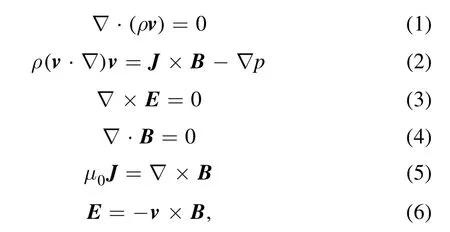
where ρ, p, v, J, B and E are the plasma density, the pressure, the plasma flow velocity, the current density, the magnetic field, and the electric field respectively.Letbe the poloidal-disk flux [29].Then, the magnetic field can be expressed aswhere BRand BZare the horizontal and vertical magnetic fields respectively.Fromμ0J= ∇×B,then

where Jφis the toroidal plasma current density and Δ* =R2∇ · (∇R2).The poloidal fulx is able to be determined by equation(7)if Jφand the boundary condition are known.In the following part, we will discuss the expression of Jφ.Faraday’s law∇×(B×v)= 0andB· (B×v)= 0implyB×v= Ω (ψ)∇ψ,where Ω(ψ)is an arbitrary function of the poloidal flux.If only a toroidal folwv=vφ eφis considered,thenB×v= ∇φ× ∇ψ×vφ eφ=(vφ R)∇ψ.We have

where Ω(ψ)is the toroidal angular velocity of the flux surface[26].Similar to the poloidal fulxψ(R,Z),we defnie a poloidal current functionand then obtainUsing ∇ ·∇×B=μ0∇·J=0,we haveand the poloidal currentJp= (∇F×eφ)μ0R.From the R component of the Ampere’s law equation(5), we getμ0JR= - (∂F∂Z)R= -∂Bφ∂Z,which implied

Considering(v· ∇)v= -RΩ2(ψ)eR,the φ component of the momentum equation reduces to(-ρv·∇v- ∇p+J×B)φ=(J×B)φ=(∇×B×B)φ=(B R) ∇(RBφ)=0,which means that the poloidal current functionF(R,Z)=RBφ=F(ψ)is also an arbitrary function of the poloidal fulx.The momentum equation is written in the following form

where prime ′ denotes∂∂.ψFrom the momentum equation,B·∇p=B· (-ρv·∇v+J×B)=ρRΩ2B·∇R≠ 0implies that the plasma pressure is not a flux surface quantity anymore.

The thermodynamic relationship of p, ρ and T in the presence of the plasma rotation are derived in two forms[20,21,25,26].The first form isp=A(S)ργ,where S(ψ)is a function of the specific entropy, which considers isotropic plasma and holds for the isentropic flowB·∇S(ψ)= 0.The other isp=T(ψ)ρ,where T is the plasma temperature, and T=T(ψ) is a surface quantity because of the large heat conductivity along the magnetic field line within a flux surface, which implies the isothermal flowB·∇T(ψ)= 0.In this work,both of the isentropic and isothermal equilibria are developed.

(1) For the isentropic case S(ψ), the right-hand side of equation (10) can be written in the following form[21, 25]:

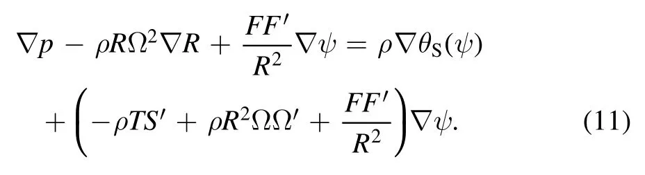
whereA′ =dA[S(ψ)]dψ.For the isentropic case,equation (12) is the general equilibrium equation of an axisymmetric plasma with a toroidal rotation in the cylindrical coordinate, where the entropy is assumed to be constant on magnetic surfaces.There are four arbitrary functionsθS(ψ),S(ψ),Ω(ψ)andF(ψ)in equation (12).If these four functions and the boundary condition are given, the solution of equation (12) is solely determined.

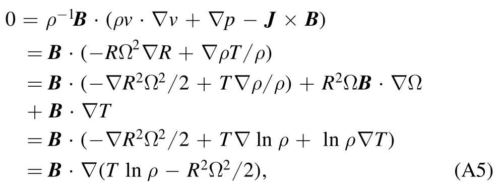
(2) For the isothermal caseT(ψ), the right-hand side of equation(10)can be written in the following form[25]:

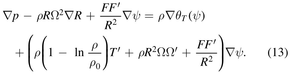
We find thatθT(ψ)= -R2Ω22+Tln (ρ ρ0)is also a surface quantity(see appendix).Equations(7)and(10)reduce to

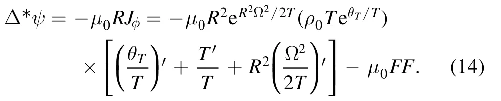
Similarly, for the isothermal caseT(ψ),the solution of equation (14) is also solely determined if the four arbitrary functionsθ T(ψ),T(ψ),Ω(ψ)andF(ψ)and the boundary condition are given.

3.The construction scheme for the free boundary conditions

In this section,both the‘divertor-type’and‘limiter-type’free boundaries are presented.A poloidal cross section of HL-2A tokamak with the divertor and the limiter is shown in figure 1.According to the plasma flux ψ or the initial flux ψ0,different regions in the computational domain are defined as follows.

First of all,the current filament method[28,30]is used to calculate the initial plasma flux ψ0in the computational domain.Specifically, the toroidal current density on the grid is regarded as a current filament and can be obtained approximately by equation (13) or (14).Then together with coil currents,ψ0is calculated by the Green’s function method.The plasma flux ψ can be obtained by iteration, which is described on section 4.The ‘main plasma’ region consists of＜1,where=(ψ-ψaxis) (ψb-ψaxis)is the normalized poloidal flux,ψaxisandψbare the flux at the magnetic axis and the‘main plasma’boundary,respectively,andψ˜ =1 represents the plasma boundary.For the divertor configuration, the boundary is the separatrix or the LCFS.For the limiter, the boundary is the isoline of the constraint point which is the interface between the plasma and the limiter.Secondly, the SOL region consists of- 1is the width of the SOL region that is roughly interchangeable with the power decay length λqthat is designed to be about 20 mm (～1.03) based on the experiment [31, 32].Thirdly, the vacuum region represents the area where the magnetic field is generated only by nonlocal currents, such as the plasma current and the external coil.Fourthly,the‘private flux’region(only for the divertor)consists of＜1 and is located below the X-point.SOL is slightly widened into the ‘private flux’ region.In reality, the plasma region is more complicated than the above definition when the divertor is considered [33].

The main plasma boundary=1 is critical for the free boundary plasma equilibrium.For the limiter-type case, the boundary is the isoline of the constraint point where the interface is between the plasma and the limiter.The plasma equilibrium is solved under the external field,as shown in figure 1(b).It is a bit more complicated for the divertor-type case.In order to produce the real divertor configuration,we need to consider divertor coils as shown in figure 1(a).Moreover, for the high beta plasma equilibrium, the plasma will shift toward the low field side.Therefore,vertical field coils are designed to generate the vertical magnetic field to push the plasma inward by the Lorentz magnetic force.The shape and the position of the plasma are consistent with these coil currents.According to the position of these external coil, two numerical methods are adopted.If external coils are located inside the computational domain, they are regarded as local plasma currents and the flux ψ can be computed through equation (16).If external coils are located outside the computational domain, the Green’s function method will be adopted via equation (19).

3.1.Current sources located inside the computational domain

Because divertor coils are located inside the computational domain for the ‘divertor-type’ free boundary, we divide the computation domain into three parts, namely the plasma region(included the main plasma and SOL),the divertor coils region,and the vacuum region(including a part of the private flux area) as shown in figure 1(a).In the plasma region, the current source is the plasma toroidal current density Jφin equation (12) or (14), so the flux function ψ satisfies equation(7).In the vacuum region,there is no current source,so the flux function ψ satisfies

In the divertor coil region, the divertor coil currents are regarded as local plasma currents.Thus, the flux function ψ satisfies

Three divertor coils, namely D1 (JD1), D2 (JD2), and D3(JD3), are designed in this scheme, and the coil currentsJDiis a parabolic distribution function.The current direction of the D1 and D3 coils must be opposite to that of the plasma current.The current direction of the D2 coil is the same as that of the plasma current.

3.2.Current sources located outside the computational domain

In this case, because the vertical/horizonal field coils located outside the computational domain as shown in figure 1, we introduce the Green’s function

where G(x, x′) is the magnetic flux at x′=(R′, Z′) produced by one Ampere vertical coil current at x=(R, Z) [27].F(k)and E(k)are the first and the second complete elliptic integrals respectively, andk2=4RR′[(R-R′)2+(Z-Z′)2].This Green’s function in equation (17) satisfies

Because the current source is located outside the computational domain, this function is reduced asΔ*G(x,x′) =0 in the computational domain.Therefore, the total poloidal flux ψ is expressed by the Green’s function in the following form.

where ψpis the contribution from the plasma current,ψicoilis the contribution from the ith external coils, andIicoilis the ith coil current.The Green’s function method can be applied to all poloidal field coils that are located outside the computational domain, for example, horizontal coils are used to control the plasma vertical displacement while vertical field coils are used to control the plasma horizontal displacement.

4.Numerical procedure

Figure 2 is the flowchart of the CLT-EQ code.The equilibrium equation is computed on a 256×256 grid of the(R,Z)plane.The solving procedure is as follows.

Figure 1.(a)For the‘divertor-type’free boundary in HL-2A tokamak,the computational domain is divided into the main plasma,SOL,the vacuum,the private-flux,and the coil region.Note that the divertor coil is located inside the computational domain.(b)For the‘limiter-type’free boundary, the computation domain is only divided into the main plasma, SOL, and the vacuum region.

Figure 2.Flowchart of CLT-EQ.

A.The four parameter functions,θS(ψ),S(ψ),Ω(ψ)andF(ψ)in equation (12) orθT(ψ),T(ψ),Ω(ψ)andF(ψ)in equation (14) are constructed.The profile of the parameter function can be chosen to be surfaceaveraged data from experiment or be specially designed for simulation requirement.Moreover, the plasma flow Ω is freely adjusted to study the effects of plasma flows on the equilibrium.

B.The initial flux ψ0is calculated via a set of external coils and the initial plasma current.ψ0is critical for convergence.And it contains information of the plasma shape and displacement.

C.The X-point, the separatrix, and the magnetic axis are calculated through the initial flux ψ0or the updated flux ψ.In other words, the position and the flux of the X-point are calculated from ψ0or ψ, and LCFS is identified through the isoline of the X-point.Then the computational domain is divided into the plasma region (including the main plasma and SOL), the vacuum region (including a part of the private flux area), and the divertor coil region.Current sources in each region are obtained via equations (12),(14)–(16).

D.Equations (7),(15),and (16) are simultaneously solved using the strongly implicit procedure method to update the magnetic flux ψ[28,34,35].In the nth iteration,the iterative formula isΔ*ψn+1= -μ0RJφ(R,ψn).The convergence defined with a condition on the residual of this formula iswhere N is the number of grids.

E.Steps C and D are iterated until the flux ψ at the end of step D remains unchanged within a given tolerance.

F.After an equilibrium calculation, we need to check whether plasma is in a reasonable position.If not,external coil currents need to be adjusted in order to obtain a suitable plasma position shown in figure 3.Meanwhile, the initial poloidal flux ψ0is recalculated at step B.Consequently, the new flux ψ is updated by iteration of steps C, D and E again.In the freeboundary calculation, the boundary condition is imposed during initialization.The X-point, the magnetic axis, and the separatrix are not fixed and determined as a part of the solution of the equilibrium problem.Figure 3 is a high beta H-mode equilibrium.In this case, vertical field coil currents produce the vertical magnetic to put the plasma inward by the Lorentz force.Otherwise, the plasma will move to the low field side due to a large thermodynamic force.We note that the boundary is a constraint by a fixed point for the limiter-type case, while the X-point is free for the divertor-type case.

Figure 3.Vertical coils to control the horizontal displacement in divertor configuration (a) and limiter configuration (b).Due to lack of vertical coils control, the plasma is not in correct position (black line).The plasma is in the correct position with reasonable vertical coils current (red line).

5.Numerical results

5.1.Benchmark with analytic solution

Benchmark tests are carried out to verify the credibility and the applicability of CLT-EQ.An exact solution of equations (12) and (14) was obtained by making the following assumptions in [21, 25]:

where P0,F0,ψ1,and M are constant.R0is a scale length.For the isentropic case, we make a further assumption of Ω2H=w2R02,and then the equation (12) is reduced as

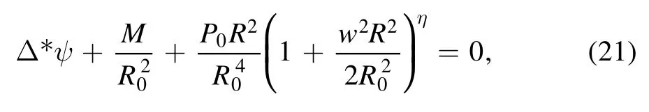
where,η=γ γ-1,w2=2M02( 2(γ- 1)-M02),M0is the Mach number at R=R0.In this benchmark case with M=0, the exact solution of equation (21) is given as the following form [21, 25]

whereG(R R0)= 1+w2R22R02,C=(εa-1)Ra28R02-(1-Gη+1) 2 (1+η)w2,Rais the magnetic axis and εais a constant and responds to plasma shape.For the isothermal case, we also make a further assumption ofΩ2=γw2R02,and equation (14) is reduced as [25]

whereis constant,w2=M02.In this benchmark case with M=0, the exact solution of equation (23) is given as the following form [25]

whereC=(εa-1)Ra28R02-(eγw2Ra22R02-1) 2γw2.To benchmark with the analytic solution mentioned above, the plasma-vacuum boundary is ignored.This means that the whole computational domain contains the plasma.The Dirichlet boundary condition is adopted.On the boundary of the computational domain, ψ is fixed and equal to the boundary magnetic flux obtained from equation (22) or (24).We use the parameters with R0=Ra=1, M0=1, εa=0 and η=5/2.Figures 4(a) and (b) show the results from analytical (black line) and numerical (read dot line) solution,which indicates that there is no visible difference of the numerical and analytical results for both the isentropic and isothermal cases.We further examine the relative error in detail by usingδ=∣(ψN,Z=0-ψA,Z=0) (ψmax-ψmin)∣that is defined to quantify the deviation between numerical and analytical solutions.ψN,Z=0andψA,Z=0are the numerical and analytical fluxes on Z=0 respectively.ψmaxandψminare the maximum and minimum values of the magnetic flux from the analytical solution respectively.Figures 4(c) and (d) indicate that the maximum deviation δ is nearly 0.1%in the region of the strong poloidal magnetic field, which suggests that the numerical solution agrees reasonably well with the analytical result.

Figure 4.Comparison of the magnetic flux obtained from the analytic (black line) and numerical (read dot line) solutions.(a) For the isentropic case, the numerical solution is calculated by equation (21), and the analytic solution is obtained by equation (22).(b) For the isothermal case,the numerical and analytic solutions are calculated by equations(23)and(24),respectively.The relative error δ is defined to quantify the deviation between the numerical and analytical solutions.(c) and (d) The isentropic and isothermal cases, respectively.

Figure 5.(a)Shafranov shift as a function of M0.Solid and dashed lines correspond to the low and high beta plasma,respectively.Red and black lines represent the isothermal and isentropic cases, respectively.(b) Magnetic flux surfaces in the presence of the high toroidal flow.The X-point is slightly shifted upward.

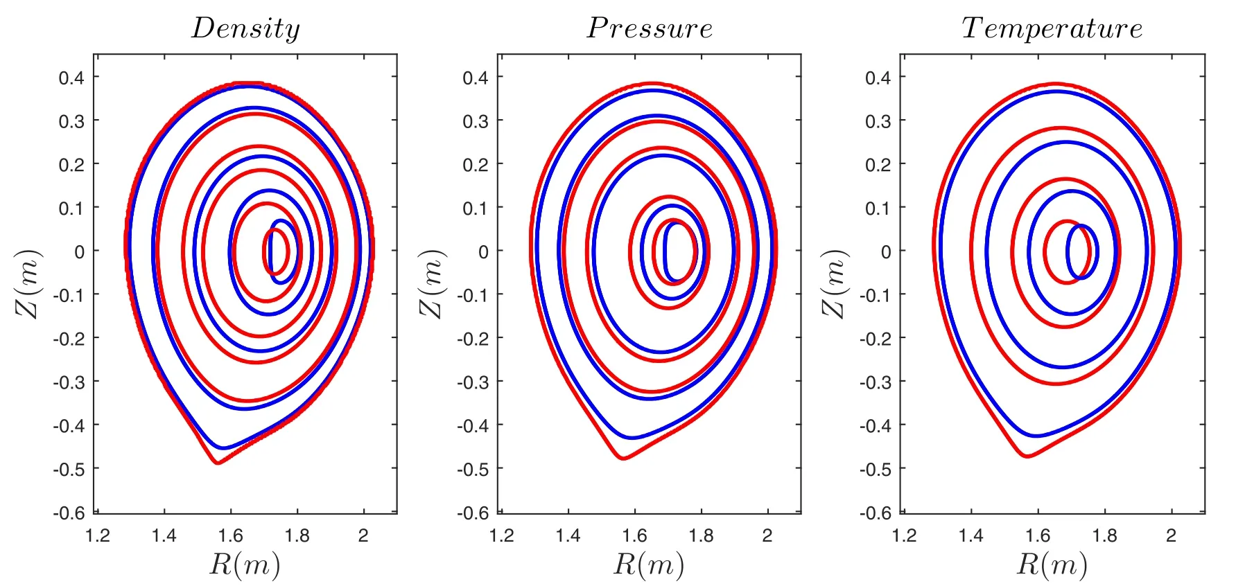
Figure 6.Contour profile of density, pressure, and temperature for isentropic (blue) and isothermal (red) cases with a high toroidal flow.

5.2.Effect of toroidal plasma flow on magnetic shift

As we know,the magnetic axis is displaced due to the plasma pressure and the internal inductance, which is named as the Shafranov shift.With the toroidal plasma rotation, the momentum equation (2) can roughly be expressed asJ×B≈∇ [p+ρ(v22) ],which means that the ‘kinetic energy’ density,ρ(v22) ,like the plasma pressure, also contributes to the Shafranov shift.In order to investigate the effect of the toroidal flow on the magnetic axis shift, we use the toroidal Alfvén Mach number,M=vφ vA,to quantify the plasma flow.vAis the Alfvén speed and M0is the toroidal Alfvén Mach number on the magnetic axis.In order to concentrate on the contribution of the toroidal flow in the Shafranov shift, we subtract the Shafranov shift in the static equilibriaΔΩ=0from the total shiftΔΩ,and normalize with the plasma minor radius a0.The expression(ΔΩ- ΔΩ=0)a0quantifies the contribution of the toroidal plasma folw to the Shafranov shift as shown in fgiure 5(a) where the red and black lines represent for the isothermal and isentropic cases, respectively.The solid and dashed lines correspond to low beta and high beta plasma,respectively.The magnetic shift is larger at a lower beta plasma or a higher M0for both isothermal and isentropic cases, which is not surprising since the‘kinetic energy’term,compared with the pressure term in the momentum equation,will become more important with the plasma beta decreasing or the toroidal flow(or M0)increasing.In addition, in the low beta plasma, the magnetic shift in the isothermal case is larger than that in the isentropic case.This difference is more severe whenM0increases.However, it is seen that the effect of the toroidal rotation on the shift in the high beta plasma is qualitatively similar for both cases.The magnetic shift due to the toroidal flow is about 0.04a0at M0=0.2.Of more interest is the shift of the X-point due to the toroidal plasma flow as shown in figure 5(b),which is only calculated in the‘divertortype’ free boundary equilibrium.The X-point is slightly shifted upward by about 0.0125a0for both the isentropic and isothermal cases at M0=0.2.In reality,M0is almost less than 0.05 for most of present tokamaks [11].Therefore, the effect of the toroidal flow on the magnetic axis and the X-point shift may be neglected.

5.3.Effect of toroidal flow on plasma parameters

The effects of the toroidal flow on plasma parameters,such as the density, the pressure, and the temperature, are shown in figure 6 where the red and blue lines represent the isothermal and isentropic cases, respectively.As we can see, centrifugal force, which is induced by toroidal flows, shifts the plasma outward, which is similar to both cases.However, since the plasma temperature only depends on the fluxT=T(ψ)in the isothermal case, the effect of the toroidal flow on the temperature should have the same effect on the magnetic shift.The temperature is expressed asT=A′ργ-1S′ (γ-1)in the isentropic case, which means that both the shifts of the temperature and density profiles should be similar.

6.Conclusion and discussion

In this paper,a free-boundary equilibrium solver(called CLTEQ)with toroidal flows and SOL is presented.There are two kinds of construction schemes for the free boundary, namely‘divertor-type’and‘limiter-type’.Different regions,including the main plasma, SOL, the vacuum, and the ‘private flux’region, are defined in the computational domain in order to design current sources.If the external coils are located outside the computational domain, the Green’s function method will be adopted.With toroidal plasma flow, the flux function is considerably different under the isentropic and isothermal assumptions.For the isentropic case, the entropyS(ψ)is constant on magnetic surfaces.Four arbitrary functionsθS(ψ),S(ψ),Ω(ψ)andF(ψ)are pre-required for an equilibrium.For the isothermal case,the plasma temperatureT(ψ)is a surface quantity due to large heat conductivity along magnetic field lines.Another four arbitrary functionsθ T(ψ),T(ψ),Ω(ψ)andF(ψ)are needed.The effects of the toroidal plasma flow on the Shafranov shift are investigated.In a high beta plasma,the magnetic shifts due to the toroidal plasma flow are almost the same for both the isentropic and isothermal cases and are about 0.04a0at M0=0.2.In addition,the X-point are slightly shifted upward by 0.0125a0.But in fact, the effect of the toroidal flow on the magnetic axis and the X-point shift may be neglected because M0is usually less than 0.05 in real tokamaks.The effects of the toroidal plasma flow on plasma parameters, such as the density, the pressure, and the temperature,are also investigated.The high toroidal flow shifts the plasma outward due to the centrifugal effect.But temperature profiles are noticeable difference in two cases because the plasma temperature is the flux function in the isothermal case.

Acknowledgments

This work was supported by National Key Research and Development Program of China(Nos.2019YFE03030004 and 2019YFE03020003),and National Natural Science Foundation of China (NSFC) (Nos.11775188 and 11835010).

Appendix

From the well-known thermodynamic relations

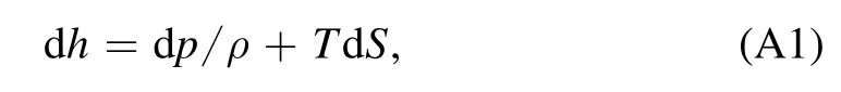
where h is the specific enthalpy.Considering the isentropic problem dS=0 and then equation of statep=A(S)ργ[21, 25], the following relation can be obtained:

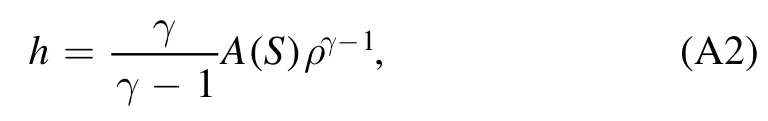
where γ is the ratio of specific heat that is chosen to be 5/3 as usual.Considering the isentropic equilibrium withv·∇S(ψ)= 0,and multiplying the momentum equation byρ-1B,the following expression is obtained by usingv·∇v= -RΩ2(ψ)∇RandB·∇Ω =0

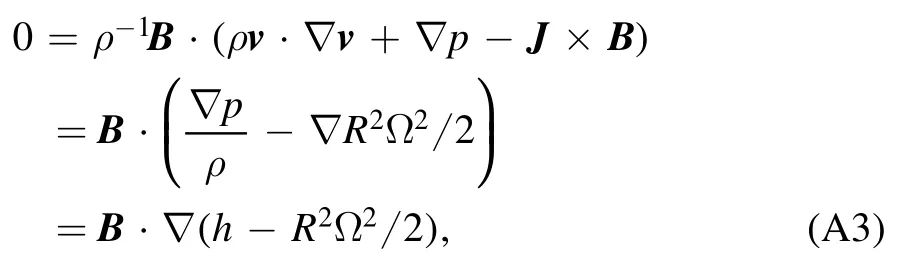
which suggests that the Bernoulli equation is an arbitrary function of the poloidal flux, i.e.

Now let us consider the isothermal equilibriumT(ψ).The plasma is assumed an ideal gas,p(R,ψ)=T(ψ)ρ(R,ψ).Multiplying the momentum equation byρ-1B,the following expression is obtained by usingv·∇v=-RΩ2(ψ)∇RandB·∇T=0

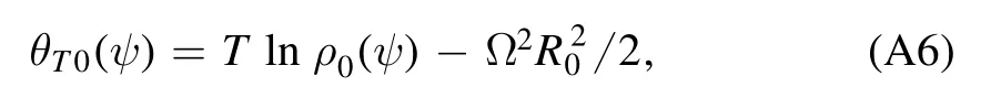
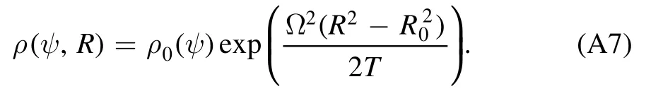
which indicates thatθT(ψ)=Tlnρ-R2Ω22orθT(ψ)=Tln(ρ ρ0(ψ))-R2Ω22is also an arbitrary function of the poloidal flux.In order to ensure the flux surface quantity ofθT(ψ),we need to carefully construct a density distribution functionρ(R,ψ).With a referenced density distributionρ0(ψ),we have

where R0is the major radius.Thus, the density that is not a flux surface quantity can be expressed as follows,

And similarly, the pressure can also be expressed to be

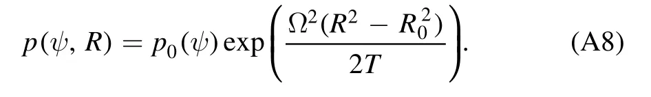
Note that the relationp0(ψ)=T(ψ)ρ0(ψ)must be satisfied.In other words, only two of the three parametersp0(ψ),ρ0(ψ)andT(ψ)can be chosen freely.θT(ψ)constructed by this method can easily be proved to be the flux surface quantity,

ORCID iDs