
Impact of thermostat on interfacial thermal conductance prediction from non-equilibrium molecular dynamics simulations
2022-05-16 07:11SongHu胡松Zhao赵长颖andXiaokunGu顾骁坤
Chinese Physics B 2022年5期
Song Hu(胡松), C Y Zhao(赵长颖), and Xiaokun Gu(顾骁坤)
Institute of Engineering Thermophysics,School of Mechanical Engineering,Shanghai Jiao Tong University,Shanghai 200240,China
Keywords: interfacial thermal conductance,phonon transport,molecular dynamics
1. Introduction
Quantitatively evaluating the roles of interfaces on phonon transport in nanoscale semiconductor structures is of primary significance for designing electronic devices with exceptional heat dissipation.[1]Microscopically, phonons are scattered by an interface made up of two dissimilar materials, and only a portion of them can transmit through the interface.[2,3]As a result, the interface result in an additional thermal resistance to heat flow other than the resistance within the material,[4]which leads to a temperature discontinuity at the interface. The heat flow across the interface,J,is linked to the temperature jump at the interface,ΔT,through

whereRis the so-called thermal boundary resistance(TBR)or Kapitza resistance,[5,6]andGis the inverse ofRand known as the interfacial thermal conductance (ITC) or thermal boundary conductance. Earlier measurements on superlattice thermal conductivity provide a way to estimate the ITC of the interfaces within the superlattice.[7,8]With the advances on pump-probe technique and electron beam heating method, it is possible to measure the interfacial thermal conductance directly.[9–13]
On theoretical side, the commonly used methods to predict the ITC can be generally classified into two groups:methods based on the Landauer formalism[14,15]and molecular dynamics (MD) simulations.[16–20]The Landauer approach requires the information of phonon transmission through an interface. Many techniques had been suggested to compute phonon transmission.[6,21–26]A common assumption of these methods is that phonon scatterings are elastic. On the other hand,it has been recognized that the inelastic effects are crucial to correctly predict the temperature dependent ITC.[27–33]For MD simulations,inelastic scatterings of phonons are naturally inherited,which make it ideal to study the ITC of various interfaces. Though both equilibrium and non-equilibrium schemes have been adopted to predict ITC,[17–20,34]the nonequilibrium molecular dynamics (NEMD) seems more popular compared with the equilibrium one,as NEMD results usually converge faster.[20]In NEMD simulations, one usually computes the ITC through Eq. (1) after setting up a temperature difference between two ends(thermal reservoirs)of the interfacial system. Both the Nose–Hoover and Langevin thermostats are frequently employed to control the temperatures of thermal reservoirs when studying ITCs.[35–37]The impacts of the temperature control methods on phonon transport properties and lattice thermal conductivity prediction from NEMD simulations have been explored by some researchers. Fillipovet al.[38]reported that the long wavelength mode phonons in Fermi–Pasta–Ulam chains will couple the two reservoirs when using the Nose–Hoover thermostat method,and they believed that the existence of the long-wavelength mode is beneficial to the energy transport. Chenet al.[39]found that the thermal reservoir parameters are critical to obtain the correct thermal properties and the Langevin method is recommended for its stochastic excitation of phonon modes. Xionget al.[40]suggested that the nonlinear part of temperature profile should not be excluded for thermal conductance calculation in NEMD simulation, and pointed out that the Nose–Hoover thermostat may produce artifacts leading to unphysical thermal rectification. Later, Huet al.[41]found different thermostats result in distinct thermal transport characteristics due to the different modal phonon excitations inside the thermostats, and lead to disparate temperature profiles. These studies concentrate on calculation of thermal conductivity, but influence of different thermostats on prediction of ITC in NEMD simulations has not received much attention yet. Barisik and Beskok[42]studied the effects of boundary treatment on NEMD simulation for solid-liquid interfacial thermal resistance and found that artificial resistance near reservoirs is dependent on the thermostat methods, however they did not report the ITC values for the solid–liquid interface. Lianget al.[34,43]found that when using the velocity rescaling method to generate temperature difference, making the reservoir wall rough can lead to correct ITC predictions by reducing the specular reflection of phonons in reservoirs. In addition, they realized that the Langevin thermostat can eliminate the specular reflection,but did not recommend the use of the Langevin thermostat as it may result in unrealistic phonon distributions if a high friction coefficient is used. However,according to the recent work by Xionget al.,[40]the Langevin thermostat can lead to reasonable thermal conductivity prediction when choosing a proper friction coefficient. The phonon transport in interfacial systems may be quite different from that in homogenous materials. For instance, whether the Nose–Hoover thermostat can assist energy transport is questionable in the interfacial system,as the abrupt structure can inhibit the propagating of the longwavelength modes. Therefore, natural questions are whether different thermostat methods result in the same ITC prediction and how much heat a specific phonon mode carry in each situation. It is also worth to elucidate the effect of atomic details in the thermal reservoirs on phonon transport in the interfacial system as this is closely relevant to the interpretation of the measured ITC in different experimental setups.
In this paper, we perform NEMD simulations to investigate phonon transport through a sharp Si/Ge interface, aiming to exploring the influence of two commonly used thermostat methods on the predicted interfacial thermal conductance from NEMD simulations. To uncover the features of phonon dynamics in inhomogeneous interfacial systems under different thermostats, we apply the spectral decomposed method to extract modal phonon temperature profiles and spectral heat flux across the interface. Our calculations show that the Nose–Hoover thermostat systematically underestimates the ITC compared with the Langevin thermostat,which is caused by the fact that the low-frequency acoustic phonons cannot be thermalized by the Nose–Hoover thermostat. This finding is opposite to the previous understanding that the coupling of long-wavelength phonons is beneficial to energy transport.In addition, we elucidate the role of atomic roughness of the thermal reservoir boundary on the interfacial thermal conductance. The introduction of epitaxial rough boundaries of the thermal reservoir is found to assist the phonon thermalization,but cannot eliminate the non-equilibrium phonon distribution in thermal reservoirs completely as the long mean-free path of acoustic modes.
2. Numerical methods
2.1. NEMD method for ITC
In this work, the MD simulations are implemented by using the Graphics Processing Units Molecular Dynamics(GPUMD)package.[44]The interfacial model is composed by connecting crystalline Si and Ge along the (100) direction as shown in Fig.1(a).Such an interfacial structure has been commonly chosen as an example to study the phonon transport through interfaces.[17,23–25,31–33,45–47]The interatomic interactions of both Si and Ge are described by the Tersoff potential for Si,[48]considering the relative small difference between their force fields.[49]The lattice constants of Si and Ge are both set as 0.5431 nm. The simulation model box have the cross section of 6×6 unit cells(UCs)with periodic boundary conditions,which is large enough to get rid of the size effects in the lateral directions.[50]A few layers of atoms are fixed at both ends of the model as shown in Fig.1(a).Next to two fixed walls,two groups of atoms within a length ofLresare coupled to hot and cold reservoirs, respectively, which are denoted as heat source and heat sink. The timestep is set as 1 fs for all of simulations,which is sufficient to eliminate the energy fluctuations and has a good resolution for phonon frequency.
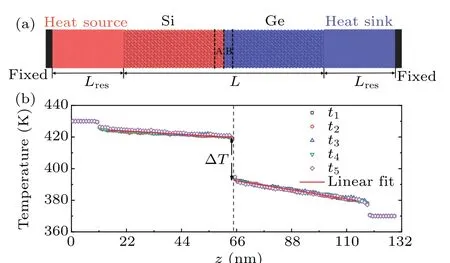
Fig.1. (a)A typical simulation system of Si/Ge interface structure for ITC prediction. (b)A typical temperature profile for the Si/Ge interfacial system at a temperature of 400 K with Langevin thermostat. The different color hollow dot represents the average temperature over different time spans by dividing the collected date into five parts. The red line is the linear fitting of the temperature profile.
During the NEMD simulations, the interfacial structure is firstly relaxed under the constant pressure and temperature(NPT) ensemble for 4 ns at the target temperatureT. Then,the system is switched to the micro-canonical (NVE) ensemble,and the temperatures in the heat and cold reservoir are set toT+T′andT-T′, respectively.T′, which is set to 30 K in our simulations, is the temperature difference between the reservoir and the average temperature of the system,the results with differentT′are also compared as shown in Table 1. This step is carried out for at least 6 ns to make the system to reach a steady state. Additional 24 ns is used to collect the data for the ITC prediction.
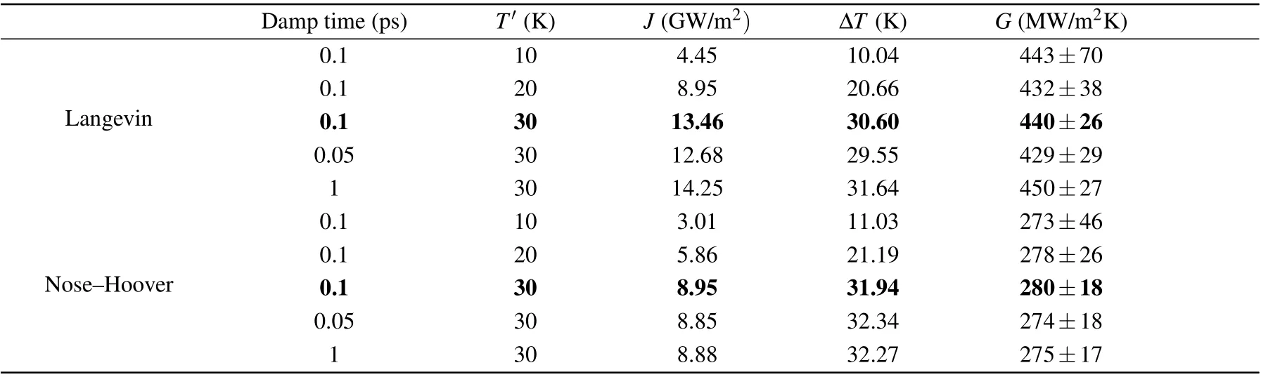
Table 1. The results obtained with different damp times of thermostats and temperature differences T′ between reservoirs,the average temperatures are set as 300 K and the length of the reservoirs is 20 UC.
Here, we concentrate on the influence of thermostat method used in the NEMD simulation. Two typical methods,the Nose–Hoover and Langevin thermostats,are adopted to control the temperatures of reservoirs. For the Langevin thermostat method,the equation of motion for particles(with massmi, forceFi, positionriand momentumpi) are governed as[37]
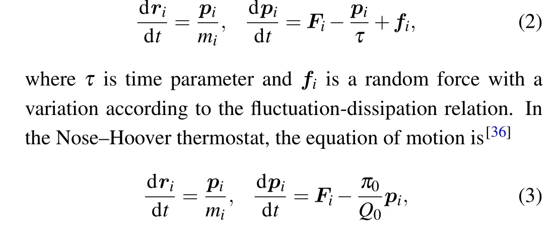
whereQ0=NfkBTτ2is the “mass” of the thermostat variable directly coupled to the system,andπ0is the corresponding “momentum”. In our simulations, the damping time of both thermostats is set as 0.1 ps, which was recommended in Ref.[40]. We also compare the results obtained from different damping times to prove this,as summarized in Table 1.
Finally, we can obtain the temperature profile as a function of position,as plotted in Fig.1(b). By linearly fitting the temperature profiles on both sides,we obtain the temperature drop ΔTat interface. The steady-state heat flux is obtained by monitoring the energy changes in the reservoirs. Then,we can calculate the ITC according to Eq. (1). It should be noticed that the linear response theory is applicable when the temperature gradient is sufficiently small.[51]It has been proved that the linear response theory should be robust and can give reasonable results if the temperature gradient is smaller than 1 K/nm.[16]The temperature gradient does not exceed this threshold in our simulations. As is seen in Table 1, the calculated ITC could not change with the temperature difference between two reservoirs if it is smaller than 30 K.
2.2. Spectral decomposed heat flux
In addition to the value of ITC, the heat flux across the interface can be spectrally decomposed using the NEMD method.[52]We define two groups of atoms,A and B,close to the both sides of the interface,as shown in Fig.1(a). The heat flux across the interface can be expressed as[53,54]

whereSis the cross-section area and ΔTis the temperature drop at the interface.
2.3. Spectral phonon temperature
To further investigate the effect of thermostat on phonon temperature in NEMD simulations, the spectral phonon temperature method developed by Fenget al.[55]is used to get phonon temperature of each phonon mode. In MD simulation, the phonon population follows the Boltzmann distribution. The energy for specified phonon mode is per phonon energy multiplying its population

where ˙Qλ(t) is the time derivative of normal mode amplitude, which can be obtained by Fourier transform of atomic displacement in real space
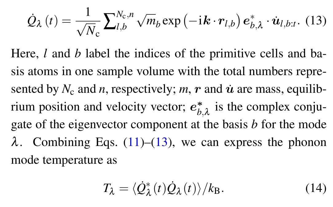
To obtain the modal temperature at different locations through Eq. (14), we divide the interfacial system into a few slabs,each of which is a supercell of 6×6×6 UCs containing 1728 atoms,and collect the atomic velocities of each slab after the steady state is achieved.
3. Results and discussion
3.1. Effect of thermostat on interface thermal conductance
Figure 2(a) shows the ITC of a sharp Si/Ge interface at 500 K from our NEMD simulations with the Nose–Hoover and Langevin thermostats as a function of length of thermal reservoirs. In these calculations, the sample lengthLis set as 200 UC (108.86 nm). Such a length is believed to sufficiently long to eliminate the size effect on the ITC of Si/Ge interface using the Langevin thermostat.[32]The calculated ITC is about 475 W/m2K and almost unaffected by the length of reservoirs using the Langevin thermostat. In contrast, for the Nose–Hoover thermostat, the obtained ITC is consistently smaller than the value from the Langevin thermostat and keeps increasing with the reservoir length even when it exceeds 80 UC. The reservoir lengths used in the previous studies fall in the length range explored here.[17,32,47]We also plot the NEMD results reported by Landry and McGaughey for comparison.[47]In their studies,the temperature difference is generated by adding and removing energy from the hot and cold reservoirs in a constant rate through a scheme of velocity rescaling(VR).Their results agree well with our results using the Nose–Hoover thermostat. Previously,Huet al.[41]noticed the equivalence between the Nose–Hoover thermostat and VR method, where they found that the Nose–Hoover thermostat and VR method lead to similar thermal conductivity prediction.
To explore how the thermostat method affects the temperature dependence of ITC,we compute ITC from 300 K to 600 K usingLres=20 UC as parameter. Figure 2(b)shows the obtained temperature dependent ITC using two thermostats,along with the NEMD results using the same size parameters reported by Landry and McGaughey. The ITC is found to increase with the temperature linearly using both thermostats,but again the ITC values with the Langevin thermostat are consistently higher than those of the Nose–Hoover one during the whole temperature range explored.To understand the origin of the discrepancy of ITC induced by the thermostat method,we examine the temperature drops at the interface (as shown in Fig. 1(b)) and heat flux along the direction perpendicular to the interface, as summarized in Table 2. All of the results are obtained at 500 K.The thermostat method as well as the length of the thermostat has little influence on the temperature drop, but the heat flux is quite sensitive. We can then focus on the discussion on the heat flux.
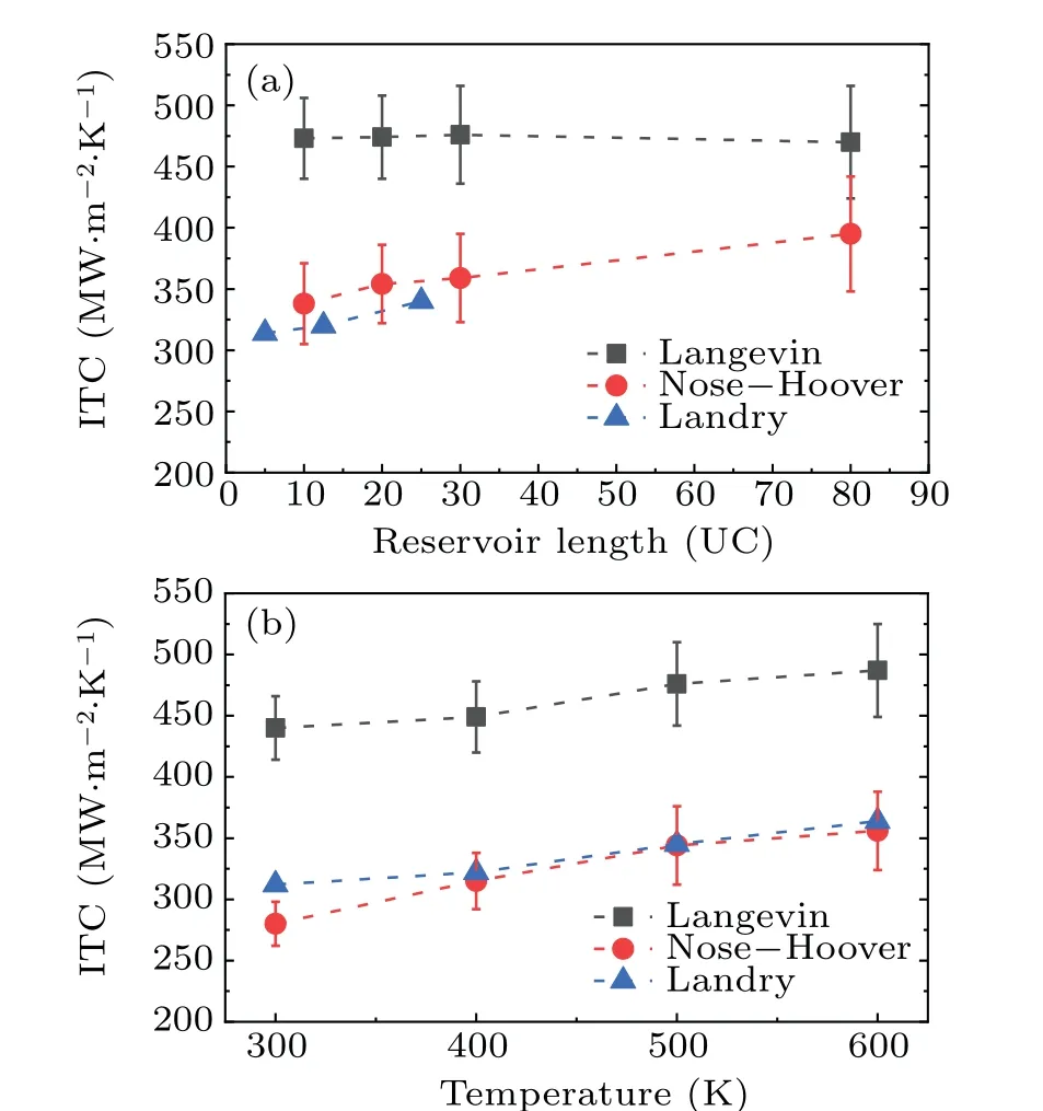
Fig.2. (a)The ITC with different reservoir lengths for the two thermostat methods at 500 K.(b)ITC obtained at different temperatures with the reservoir length of 20 UC.The blue dots are the values presented in Ref.[47].
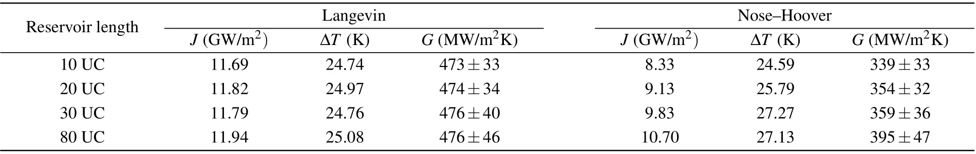
Table 2. The apparent heat flux and temperature drop for ITC calculation,with the average temperature taken as 500 K.
3.2. Analysis on spectral heat flux and modal temperature
To gain more insight into the heat flux between two thermostat methods,we compute the heat flux across the interface contributed by phonons with different frequencies using the spectral decomposed method, as shown in the Fig. 3(a). The length of the thermal reservoirs is set to 20 UC,as an example.A cutoff around 10 THz can be clearly identify, above which the spectral heat flux with both methods are almost zero, expect two small regions around 12.5 THz and 15 THz. This cutoff should correspond to the cutoff frequency of Ge. According to the mismatch models as well as atomistic Green’s function under the harmonic approximation,the phonons with frequency larger than 10 THz in Si cannot transmit through the interface, as there are no phonons with similar frequency on the Ge side to match the incoming phonons. The heat flux contributed by the phonons with frequency larger than 10 THz should be resulted from the anharmonic effects of lattice vibration.[31,56]

Fig.3. The decomposed heat flux: (a)the Langevin and Nose–Hoover with Lres=20 UC,(b)Langevin thermostat and(c)Nose–Hoover thermostat with different reservoir lengths.
When the frequency is below 10 THz, the decomposed heat flux is distinct between the two thermostat methods. Depending on the phonon frequency,the spectral heat flux can be classified into three regimes based on the distinction between two thermostat methods. (1)For the frequency below 1 THz,the Nose–Hoover thermostat induced heat flux is almost zero,but these low-frequency phonons using the Langevin thermostat still have contribution to the heat flux. (2) For phonons with the frequency from 1 THz to 6 THz,the spectral heat flux with Langevin is considerably larger than the Nose–Hoover one. (3) When the phonon frequency is larger than 6 THz,there is no significant difference between the two thermostat methods. We also examine how the length of thermal reservoirs alter the spectral heat flux, as shown in Figs.3(b)–3(c).Changing the length of thermal reservoirs with the Langevin thermostat does not lead to significant change on the spectral heat flux, which is consistent with our observation that using the Langevin thermostat the calculated ITC is independent of the length of reservoir. However, for the Nose–Hoover thermostat, the heat flux increases with the reservoir length from 10 UC to 80 UC.According to the above observation on spectral heat flux,low-and-middle-frequency phonons are believed to make the ITC values quite different between two thermostat methods.
Since heat flow is driven by temperature gradient, the smaller flux of low-and-middle-frequency phonon may result from the fact that temperature difference of these phonons is smaller than that of the high-frequency phonon. To observe the transport properties of different phonons,we compute the modal temperature along the direction perpendicular to the interface through the spectral phonon temperature method. Here we calculate the modal temperature for 162 phonon modes and plot the average temperatures for six phonon branches.Figure 4(a)shows the temperature profiles of phonons on different branches calculated from NEMD simulations using the Langevin thermostat. In each reservoir (shadow region in Fig.4),all phonons are of the same temperatures,which equal to the target temperature. At the edge between the reservoir and the interfacial region,an abrupt temperature jump can be identified for each group of phonons,which is regarded as the thermal resistance between reservoirs and the middle lead.[42]The temperature jumps of LA,TA1 and TA2 phonons are noticeably larger than those of optical phonons. In the lead region, the modal temperatures of these phonons are different,which reflects that the phonon transport is in non-equilibrium state.
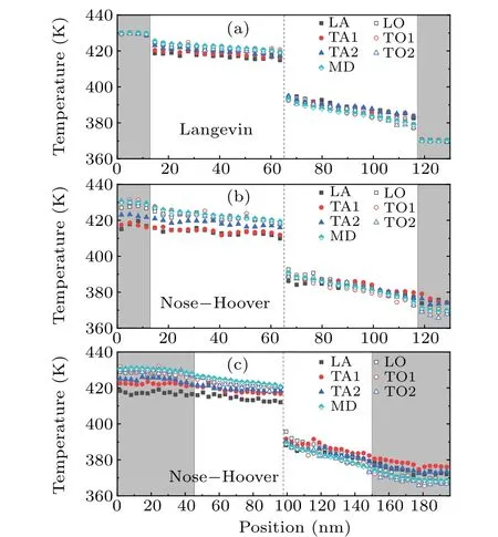
Fig. 4. The temperature profile for six phonon branches. (a) The Langevin thermostat (b) Nose–Hoover thermostat with Lres =20 UC.(c)The Nose–Hoover thermostat with Lres=80 UC.
Figure 4(b) shows the obtained temperature profile using the Nose–Hoover thermostat. Similar to the results of the Langevin thermostat, the modal temperatures of different branches in the lead are also distinct. Moreover, we can identify that even in the reservoirs the modal temperatures are not the same either. The acoustic phonons have higher(lower)temperatures compared with the optical modes in the cold (hot) reservoirs, though the average temperature of the reservoir is kept to the target temperature. Such a difference between the Langevin and Nose–Hoover thermostat on the modal temperature in the reservoirs has also been reported before on thermal conductivity prediction using the NEMD simulations.[40,41]The Langevin thermostat behaviors like an equilibrium reservoir,and all phonons that flow into the reservoir are thermalized to the target temperature within a few periods of damping time. In contrast,the Nose–Hoover thermostat only make the average temperature of the whole reservoir at the given temperature, thus the different phonons are not necessarily thermalized at the same pace.
An interpretation for the small temperature difference for acoustic phonons when using the Nose–Hoover thermostat is as follows. These phonons are of long mean-free path and large phonon transmissivity through the interface (close to unity), and therefore they can travel from one reservoir to the other one almost without scattering with other phonons and the interface. This phenomenon is closely related to the findings by Filipovet al.[38]that the long wavelength mode in the Fermi–Pasta–Ulam chain makes the two thermal reservoirs couple. A direct outcome is that after emitted from the hot(cold)reservoir,these low-frequency phonons do not sufficiently exchange energy with other phonons so that they are of higher(lower)temperature when reaching the cold(hot)reservoir. We could qualitatively regard the Nose–Hoover thermostat as an additional source of scatterings to phonons,and expect that the phonons can gain or lose energy to the reservoir due to such scatterings. However,typically the Nose–Hoover thermostat is weak, and the resultant strength of scattering to phonons is so weak to reduce the mean free path of these phonons considerably. As a result,the mean free path of these phonons is still much longer than the distance that phonons travel in the reservoir. In other words, they cannot be fully thermalized in the reservoir. For optical phonons,due to their relatively short intrinsic mean free path,they experience multiple collisions with other phonons when traveling from one reservoir to the other, making their temperature close to the local temperature. Therefore, in the hot (cold) reservoir, the acoustic phonons are usually of lower (higher) temperature than optical ones. Furthermore,though the thermal reservoirs are coupled when using the Nose–Hoover thermostat,the energy transport through the interface is not enhanced because of the small temperature difference of the acoustic modes. This observation is opposite to hypothesis by Filipovet al.[38]that long-wavelength modes in the system assist the energy transport in a homogenous system.
To clarify the effects of the reservoir size on the ITC when using the Nose–Hoover thermostat,we plot the phonon modal temperature withLresis 80 UC, as shown in Fig. 4(c). Compared with the shorter reservoir(Fig.4(b)),the phonons on TA branch have higher temperature in the hot reservoir,as the temperature gap between optical phonons and TA phonons narrowed. This means that the TA branch phonons emitted from the hot reservoir carry more energy. Therefore, the heat flux contribution from the middle frequency phonons is increased as we observe from Fig.3(c).Such a change on modal temperature of TA modes in the reservoir should be caused by the fact that the transport of TA phonons in the reservoir transits from ballistic to diffusive. As the length of reservoirs increases,the distance that phonons travel in the reservoir becomes comparable to the effective phonon mean free path. Unlike the TA modes, the phonons on LA branch still have lower temperature than other branch phonons. This is probably because they have longer mean free path than the TA modes. The distinct behaviors of phonons on different branches explain why the ITC values increase with length of thermal reservoirs but are still lower than the Langevin results.
We notice that in a previous study[34]the authors realized that the VR method(which should be equivalent to the Nose–Hoover method) with smooth fixed wall leads to strong size effect. They proposed an epitaxial rough boundary to make the phonons scattered diffusively at the fixed wall,and showed that the rough surface dramatically reduces the effects of the lead length on the ITC.According to our previous discussion,we expect that the inclusion of roughness on the fixed wall cannot eliminate the size effects on ITC completely,since the phonon scattering at the wall diffusively does not necessarily mean that phonon transport is diffusive. When a phonon hits a smooth wall,the specular scattering is expected to happen and the incoming phonon is converted to a phonon with an opposite momentum. If the wall becomes rough,the diffusive scattering at the wall likely will occur. As a result, the traveling direction of the reflected phonon will be rather arbitrary. As the phonon-fixed wall scattering is elastic and thus the energy(frequency) of phonons before and after the scattering does not change, the existence of the fixed wall does not change the spectral temperature. Hence,these phonons are still of different temperatures compared with the target temperature and are in non-equilibrium state. To quantitatively investigate the role of wall roughness on the ITC, we recalculate the spectral heat flux of the interfacial system by letting the wall be rough,as shown in Fig.5. The heat flux conducted by middlefrequency phonons is enhanced to some extent but is smaller than the Langevin thermostat, which indicates that the suggested rough wall could enhance(reduce)phonon temperature of these phonons in the hot (cold) reservoir. This is probably caused by the fact that the roughness effectively increases the distance that phonon travels in the reservoir due to multiple phonon-wall scatterings,as illustrated in Fig.5(a).However,it is found that low-frequency phonons still have negligible contribution to the interfacial thermal conductance. Again, this should be due to the longer mean free path of low frequency phonons. As the size of the interfacial region increases, the obtained ITC should increase as a longer system tends to thermalize phonons more effectively due to multiple phonon scatterings. To verify this, we compute a system with 300 nm thickness at 400 K. The obtained ITC with the Nose–Hoover thermostat is about 0.41 GW/m2K,which is larger than that in our previous structure (108 nm, 0.33 GW/m2K), as shown in Fig. 2(b). This value is still smaller than the results obtained using the Langevin thermostat(0.46 GW/m2K for both a 108 and 300 nm long system).If the system is large enough,we expect that the Nose–Hoover and Langevin thermostat will lead to the same ITC prediction. However,for materials with long phonon mean-free path(e.g.,silicon),the required size of the simulated interfacial system to achieve convergence could be as long as several microns. Hence,the Langevin thermostat is recommended in most simulations.
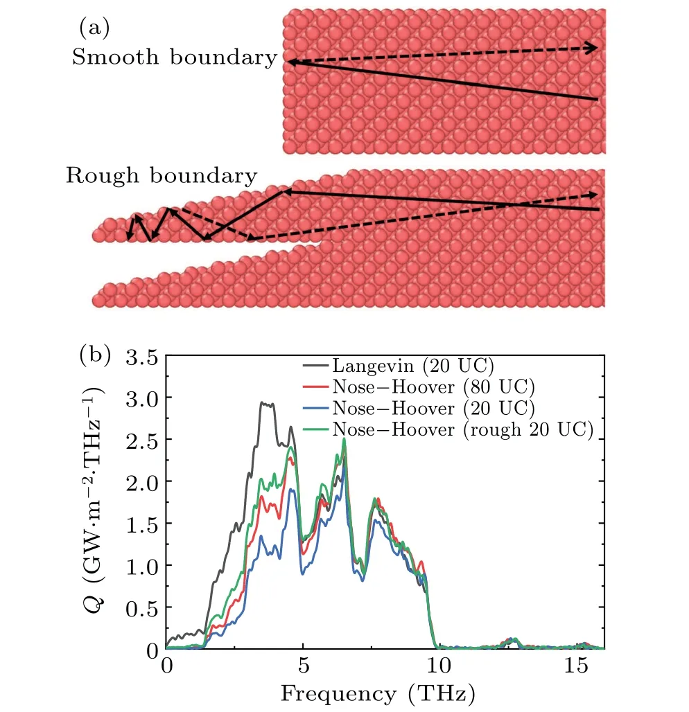
Fig.5. (a)The phonons travel in the reservoirs with smooth and rough wall. (b)The decomposed heat flux for Langevin thermostat and Nose–Hoover thermostat method with different reservoir lengths and rough wall.
4. Conclusions
In summary, we have investigated the influence of two commonly used thermostat methods in NEMD simulations for ITC prediction. In our simulations,the obtained ITC of Si/Ge interface using the Langevin thermostat is larger than the Nose–Hoover one. In addition, the results with the Langevin thermostat seem more robust than the Nose–Hoover method,which is found to be dependent on thermal reservoir length.By performing the spectral decomposed heat flux and spectral phonon temperature analysis,we find that the underestimation of the ITC values using the Nose–Hoover thermostat is caused by the small temperature difference of acoustic phonons between two reservoirs. The long mean free path and large phonon transmissivity of low-frequency acoustic phonons is suggested to be responsible. We also analyze how the roughness of the fixed wall on the ITC when using the Nose–Hoover thermostat. The inclusion of wall roughness could help to thermalize middle-frequency phonons but cannot enhance the contribution of low-frequency phonon to the ITC due to their long mean free path. Based on our results,we recommend the Langevin method in NEMD simulation when studying phonon transport through interfaces.
Acknowledgements
X.G.acknowledges the support from the National Natural Science Foundation of China (Grant No. 51706134). The computations in this paper were run on theπ2.0 cluster supported by the Center for High Performance Computing at Shanghai Jiao Tong University.

- Chinese Physics B的其它文章
- A nonlocal Boussinesq equation: Multiple-soliton solutions and symmetry analysis
- Correlation and trust mechanism-based rumor propagation model in complex social networks
- Gauss quadrature based finite temperature Lanczos method
- Experimental realization of quantum controlled teleportation of arbitrary two-qubit state via a five-qubit entangled state
- Self-error-rejecting multipartite entanglement purification for electron systems assisted by quantum-dot spins in optical microcavities
- Pseudospin symmetric solutions of the Dirac equation with the modified Rosen–Morse potential using Nikiforov–Uvarov method and supersymmetric quantum mechanics approach